Subtract the mean and divide by the standard deviation and any variable gets mean 0 and variance 1. Prove that μ and σ² are the mean and variance of N(μ, σ²), read a distribution’s lean and tails from E[Z³] and E[Z⁴], and see why the mean is the best guess under squared error.
M06.7.4L1 Core25 minIn review (what this means)
The maths and code on this page are checked by automated tests on every change, but an independent reader has not signed it off yet. Spot a mistake or a confusing step? Tell us.
Standardise a random variable as Z = (X − μ)/σ and prove that Z has mean 0 and variance 1 whatever the distribution of X.
Prove that a standard normal variable has mean 0 and variance 1, using symmetry and integration by parts, and conclude that N(μ, σ²) has mean μ and variance σ².
Compute raw and central moments, and the skewness E[Z³] and kurtosis E[Z⁴], by hand for a small PMF and with scipy.stats on samples.
Derive E[(X − c)²] = Var(X) + (μ − c)² and explain why the mean is the best single guess under squared error.
The question
A data set records waiting times in minutes and incomes in pounds. Before training, almost every pipeline rescales each column so that it has mean 0 and standard deviation 1. What does that rescaling keep, what does it throw away, and once two variables share a mean and a spread, which numbers still tell their shapes apart?
From the last lesson
1. What are \({\operatorname{Var}(aX + b)}\) and the standard deviation of \({aX + b}\)?
Show answer
\({a^2 \operatorname{Var}(X)}\) and \({\abs{a}\,\sigma_X}\); the shift \(b\) changes neither.
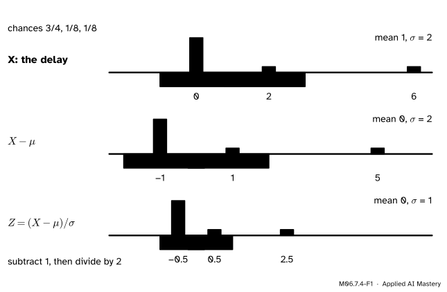
This lesson’s running example is a train’s delay \(X\), in minutes: on time (0) with probability \(3/4\), 2 minutes late with probability \(1/8\), and 6 minutes late with probability \(1/8\). Its mean is 1 minute and its standard deviation 2 minutes. To standardise it, make two moves: slide it so the mean sits at 0, then squeeze it so the standard deviation is 1.
M06.7.4-F1
Standardising in two moves. Subtracting the mean moves the pivot to 0; dividing by the standard deviation makes the band run from \(-1\) to 1. The bars keep their heights and their order: the shape is untouched.
The standardised value \({Z = (X - \mu)/\sigma}\) says how many standard deviations \(X\) lies from its mean: the 6-minute delay has \({z = 2.5}\). Every standardised variable has mean 0 and spread 1, so what is left to compare is shape: the long right tail of this delay is still there in \(Z\).
Build it up
Step 1. Why mean 0 and variance 1.\({Z}\)\({= \tfrac{1}{\sigma}X - \tfrac{\mu}{\sigma}}\) is a shift and a stretch, \({aX + b}\) with \({a = 1/\sigma}\) and \({b = -\mu/\sigma}\). By linearity and the rule for \({\operatorname{Var}(aX + b)}\),
Nothing about the shape of \(X\) was used: this holds for every \(X\) with \({\sigma > 0}\).
Step 2. Moments. The \(k\)-th moment of \(X\) is \({\E[X^k]}\), and the \(k\)-th central moment is \({\E[(X - \mu)^k]}\). The first moment is the mean; the second central moment is the variance. The third and fourth central moments carry information about shape.
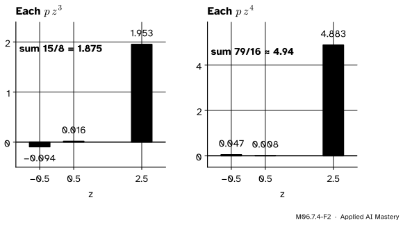
Step 3. Cubes keep the sign. A cube is negative on the left of the mean and positive on the right, and it grows fast: a value 2.5 standard deviations out contributes \({2.5^3 \approx 15.6}\) times its probability, a value half a standard deviation out only \({0.125}\) times. So the third moment is pulled towards whichever side has the long tail.
M06.7.4-F2
The third and fourth powers of \(z\) for the delay, each weighted by its probability. The rare 6-minute delay, at \({z = 2.5}\), supplies almost all of both sums.
Step 4. Standardise first, so the numbers have no units. A third central moment is in minutes cubed and changes if we switch to seconds. Taking the moments of \(Z\) instead gives pure numbers that compare shapes across any units.
The formal statement
NoteDefinition: skewness and kurtosis
For \(X\) with mean \(\mu\), standard deviation \({\sigma > 0}\) and \({Z = (X - \mu)/\sigma}\), \[
\text{skewness} = \E[Z^3],
\]\[
\text{kurtosis} = \E[Z^4].
\] Equivalently, \({\E[(X - \mu)^3]/\sigma^3}\) and \({\E[(X - \mu)^4]/\sigma^4}\).
Positive skewness means a longer tail on the right; negative, on the left; a distribution that is symmetric about its mean has skewness 0. Kurtosis is never below 1, because \({\E[Z^4] - (\E[Z^2])^2}\) is the variance of \(Z^2\); it is large when rare values sit far out in the tails. The normal distribution is the yardstick, with skewness 0 and kurtosis 3, so kurtosis minus 3, the excess kurtosis, is often reported instead.
The normal distribution’s mean and variance. Lesson M06.6.4 built \({N(\mu, \sigma^2)}\) as the standard bell \({\phi(z)}\)\({= e^{-z^2/2}/\sqrt{2\pi}}\) shifted by \(\mu\) and stretched by \(\sigma\). We can now check that \(\mu\) and \(\sigma^2\) really are its mean and variance.
Mean of \(Z\). The integrand \({z\,\phi(z)}\) is odd: \({\phi(-z) = \phi(z)}\), so the value at \(-z\) is minus the value at \(z\). Since \({\phi'(z) = -z\,\phi(z)}\), the right half is
which is finite, and the left half is its negative. So \({\E[Z] = 0}\).
Variance of \(Z\). With \({\E[Z] = 0}\), \({\operatorname{Var}(Z)}\)\({= \E[Z^2]}\)\({= \int z^2\,\phi(z)\,dz}\). Integrate by parts (M04.7) with \({u = z}\) and \({dv = z\,\phi(z)\,dz}\), so \({du = dz}\) and \({v = -\phi(z)}\):
The boundary term vanishes because \({e^{-z^2/2}}\) shrinks far faster than \(z\) grows, and the last integral is the total area under a density. Then \({X = \mu + \sigma Z}\) has \({\E[X]}\)\({= \mu + \sigma \cdot 0}\)\({= \mu}\) and \({\operatorname{Var}(X)}\)\({= \sigma^2 \cdot 1}\)\({= \sigma^2}\).
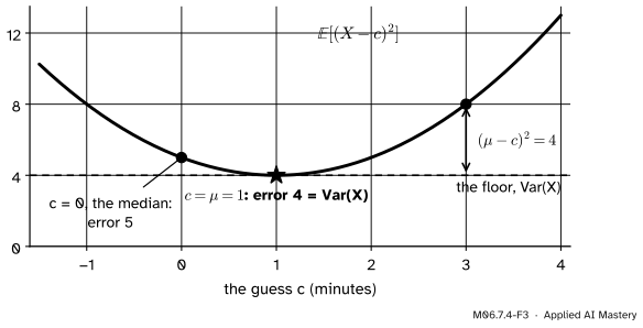
The best single guess. Suppose you must predict \(X\) with one number \(c\) and pay the squared error \({(X - c)^2}\). Write \({X - c}\)\({= (X - \mu) + (\mu - c)}\), square, and take expectations; the middle term has the factor \({\E[X - \mu] = 0}\):
The first term does not depend on \(c\) and the second is never negative, so the expected squared error is smallest, and equal to the variance, exactly at \({c = \mu}\).
M06.7.4-F3
The expected squared error of the guess \(c\) for the train delay: \({4 + (1 - c)^2}\). Its floor is the variance, 4, reached only at the mean. The median, 0, costs 5.
This is why the mean is the answer to “best constant prediction under squared error”, the starting point of regression in ML01.4.1. Under absolute error the best guess is a median instead.
Go deeper: one function that holds every moment
The moments \({\E[X], \E[X^2], \E[X^3], \dots}\) can be packed into a single function, \({M(t) = \E[e^{tX}]}\), whose \(k\)-th derivative at \({t = 0}\) is \({\E[X^k]}\) whenever \(M\) is finite near 0. For a variable with finitely many values, the moments pin the distribution down completely. That function, the moment generating function, is the subject of M07.2.
Worked example
The train delay, by hand. Mean and variance from raw moments:
The standardised values are \({z = (x - 1)/2}\): \({-1/2}\), \({1/2}\) and \({5/2}\). As a check, \({\E[Z]}\)\({= -\tfrac38 + \tfrac1{16} + \tfrac5{16}}\)\({= 0}\) and \({\E[Z^2]}\)\({= \tfrac{3}{16} + \tfrac{1}{32} + \tfrac{25}{32}}\)\({= 1}\). Now the third and fourth powers:
The delay’s skewness and kurtosis, value by value. The last row adds each column.
The skewness \({15/8 = 1.875}\) is positive: a long tail to the right, the rare 6-minute delay. The kurtosis \({79/16 \approx 4.94}\) is above the normal’s 3 (excess \({1.94}\)): more of the spread comes from rare far values than in a bell.
Code
From scratch with exact fractions.
from fractions import Fractiondelay = {0: Fraction(3, 4), 2: Fraction(1, 8), 6: Fraction(1, 8)}E =lambda g: sum(g(x) * p for x, p in delay.items()) # E[g(X)] for the delayraw = [E(lambda x, k=k: x ** k) for k in (1, 2, 3, 4)]mu = raw[0]central = [E(lambda x, k=k: (x - mu) ** k) for k in (2, 3, 4)]sigma =2# sqrt of the variance 4, exactz =lambda x: (x - mu) / sigmamoments_of_z = [E(lambda x, k=k: z(x) ** k) for k in (1, 2, 3, 4)]print("raw moments E[X^k], k = 1..4:", raw)print("central moments, k = 2..4: ", central)print("E[Z], E[Z^2], skewness, kurtosis:", moments_of_z)print("best guess c: E[(X - c)^2] for c = 0, 1, 3:", [E(lambda x, c=c: (x - c) **2) for c in (0, 1, 3)])
raw moments E[X^k], k = 1..4: [Fraction(1, 1), Fraction(5, 1), Fraction(28, 1), Fraction(164, 1)]
central moments, k = 2..4:    [Fraction(4, 1), Fraction(15, 1), Fraction(79, 1)]
E[Z], E[Z^2], skewness, kurtosis: [Fraction(0, 1), Fraction(1, 1), Fraction(15, 8), Fraction(79, 16)]
best guess c: E[(X - c)^2] for c = 0, 1, 3: [Fraction(5, 1), Fraction(4, 1), Fraction(8, 1)]
Now with samples and scipy.stats. By default scipy.stats.kurtosis reports the excess kurtosis, \({\E[Z^4] - 3}\); pass fisher=False for \({\E[Z^4]}\) itself. Both functions use the sample’s own mean and standard deviation, so on 200,000 draws they land near the exact values.
import numpy as npfrom scipy import integrate, statsrng = np.random.default_rng(4)x = rng.choice([0, 2, 6], p=[0.75, 0.125, 0.125], size=200_000)zs = (x - x.mean()) / x.std()print("standardised sample: mean", zs.mean().round(6), " sd", zs.std().round(6))print("skew:", stats.skew(x).round(3), " kurtosis:", stats.kurtosis(x, fisher=False).round(3)," excess:", stats.kurtosis(x).round(3))phi =lambda t: np.exp(-t * t /2) / np.sqrt(2* np.pi)print("E[Z^2] for the normal, by quad:", integrate.quad(lambda t: t * t * phi(t), -np.inf, np.inf)[0])print("scipy.stats.norm mean, var, skew, excess kurtosis:", stats.norm.stats(moments="mvsk"))
standardised sample: mean 0.0  sd 1.0
skew: 1.874   kurtosis: 4.941   excess: 1.941
E[Z^2] for the normal, by quad: 1.000000000000001
scipy.stats.norm mean, var, skew, excess kurtosis: (np.float64(0.0), np.float64(1.0), np.float64(0.0), np.float64(0.0))
Notice that scipy.stats.norm reports a kurtosis of 0 for the normal: it is the excess. Always check which convention a library uses before comparing kurtosis values.
Explore
The balance beam in lesson M06.7.3 shows standardising as button presses. Choose the “Even” start, whose mean is 3 and standard deviation 2, and press \({a = 1/2}\): the band now reaches one unit either side of the pivot. Two presses of \({b - 1}\) bring the pivot to \(-0.5\) (exact standardising would shift by \(-1.5\)). The bars keep their shape throughout.
Pitfalls
M06.7.4-F5
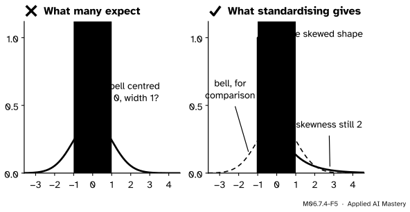
Standardising the waiting time with rate 0.5 (mean 2, standard deviation 2). The result has mean 0 and standard deviation 1, but it is the same lopsided exponential shape, now starting at \({z = -1}\), not a bell.
“Standardising makes the data normal.”
Standardising is a shift and a stretch. It changes the mean to 0 and the standard deviation to 1 and changes nothing else: skewness and kurtosis are exactly the same for \(X\) and \(Z\), because they are defined from \(Z\). A feature scaler in a machine-learning pipeline puts features on the same scale; it does not remove skew or outliers. Statements such as “95% of values lie within 2” hold for a normal \(Z\), not for every \(Z\).
“A kurtosis of 0 means the distribution is flat.”
It depends on the convention. scipy.stats.kurtosis and scipy.stats.norm.stats report the excess, \({\E[Z^4] - 3}\), so the normal scores 0; this lesson’s \({\E[Z^4]}\) gives it 3. And kurtosis is about the tails, far from the mean, not about how pointed the peak looks.
“The median is as good a single guess as the mean.”
Under squared error, no guess beats the mean, and any other guess costs exactly \({(\mu - c)^2}\) more. For the delay, the median 0 has expected squared error 5 against the mean’s 4. Under absolute error the ranking flips. Choosing a loss is choosing which summary you are estimating.
Check yourself
Recall
1. What are the mean and variance of \({Z = (X - \mu)/\sigma}\), and why?
Show answer
0 and 1: \(Z\) is \({aX + b}\) with \({a = 1/\sigma}\) and \({b = -\mu/\sigma}\), so \({\E[Z]}\)\({= \mu/\sigma - \mu/\sigma}\)\({= 0}\) and \({\operatorname{Var}(Z)}\)\({= \sigma^2/\sigma^2}\)\({= 1}\).
2. Define the skewness and the kurtosis of \(X\).
Show answer
\({\E[Z^3]}\) and \({\E[Z^4]}\), where \(Z\) is the standardised \(X\).
3. What are the skewness and kurtosis of a normal distribution?
Show answer
0 and 3 (an excess kurtosis of 0).
4. Which step proves \({\operatorname{Var}(Z) = 1}\) for a standard normal \(Z\)?
Show answer
Integration by parts with \({u = z}\) and \({dv = z\,\phi(z)\,dz}\): the boundary term is 0 and what is left is \({\int \phi = 1}\).
5. What is \({\E[(X - c)^2]}\), and which \(c\) makes it smallest?
Show answer
\({\operatorname{Var}(X) + (\mu - c)^2}\), smallest at \({c = \mu}\), where it equals the variance.
Exercises
1.★ Exam marks have mean 70 and standard deviation 10. What is the standardised value of a mark of 85, and which mark has \({z = -0.5}\)?
Show solution
\({z = (85 - 70)/10 = 1.5}\). A mark with \({z = -0.5}\) is \({70 - 0.5 \times 10 = 65}\).
2.★★ Show that a standard normal \(Z\) has kurtosis \({\E[Z^4] = 3}\).
Show solution
Integrate by parts with \({u = z^3}\) and \({dv = z\,\phi(z)\,dz}\), so \({du = 3z^2\,dz}\) and \({v = -\phi(z)}\):
using \({\E[Z^2] = 1}\) from the lesson, and \({z^3 e^{-z^2/2} \to 0}\) at both ends.
3.★★★ A test example is answered correctly with probability \(p\); let \(X\) be 1 if it is correct and 0 if not. Show that the skewness of \(X\) is \({(1 - 2p)/\sqrt{p(1 - p)}}\), and evaluate it at \({p = 0.9}\).
Show solution
The mean is \(p\) and \({\sigma^2 = p(1 - p)}\). The third central moment is
Dividing by \({\sigma^3 = (p(1 - p))^{3/2}}\) gives \({(1 - 2p)/\sqrt{p(1 - p)}}\). At \({p = 0.9}\) this is \({-0.8/0.3}\)\({= -8/3}\)\({\approx -2.67}\): a long tail to the left, the rare mistakes.
Summary card
Standardise to compare shapes; the third and fourth moments describe them.
M06.7.4-F1
Subtract the mean, divide by the standard deviation.
\({Z = (X - \mu)/\sigma}\) has mean 0 and variance 1, and the same shape as \(X\).
Normal:\({\E[Z] = 0}\) by symmetry and \({\E[Z^2] = 1}\) by parts, so \({N(\mu, \sigma^2)}\) has mean \(\mu\), variance \(\sigma^2\).
Skewness\({\E[Z^3]}\), kurtosis\({\E[Z^4]}\); normal: 0 and 3.
\({\E[(X - c)^2]}\)\({= \operatorname{Var}(X) + (\mu - c)^2}\): the mean is the best guess.
Sources and next steps
Sources. Each was opened and checked against this lesson on 14 November 2026.
Charles M. Grinstead and J. Laurie Snell, Introduction to Probability, second edition. Section 6.3, Example 6.27: the standard normal has mean 0 by symmetry and variance 1 by integration by parts, and \({X = \sigma Z + \mu}\) then has mean \(\mu\) and variance \(\sigma^2\). Section 10.1 defines the \(k\)-th moment \({\mu_k = \E(X^k)}\).
NIST/SEMATECH, Measures of Skewness and Kurtosis, e-Handbook of Statistical Methods, Section 1.3.5.11: skewness and kurtosis from the third and fourth central moments over \({s^3}\) and \({s^4}\), the normal’s values 0 and 3, the excess convention, and kurtosis as a measure of heavy or light tails.
SciPy, scipy.stats.skew (the coefficient \({m_3/m_2^{3/2}}\) from the sample’s own moments) and scipy.stats.kurtosis (fisher=True by default, which subtracts 3 so that the normal gives 0).
Next. Module M06.8 meets the named distributions, each with its mean and variance found by the rules of this module, starting with M06.8.1 Bernoulli and binomial. Correlation (M06.10.3) is the covariance of two standardised variables.