Changing units moves and stretches a density, and a stretch must lower it to keep the area 1. Derive the rule from the CDF, then meet the standard normal bell, its shifted and stretched family N(μ, σ²), z-scores and the 68, 95, 99.7 rule.
M06.6.4L1 Core25 minIn review (what this means)
The maths and code on this page are checked by automated tests on every change, but an independent reader has not signed it off yet. Spot a mistake or a confusing step? Tell us.
Derive F_Y(y) = F_X((y − b)/a) and f_Y(y) = f_X((y − b)/a)/a for Y = aX + b with a > 0, and explain why a stretch lowers a density.
State the standard normal density φ and CDF Φ, and build N(μ, σ²) as the standard bell shifted by μ and stretched by σ.
Turn a normal probability into a z-score question and answer it with Φ, using the 68, 95, 99.7 rule as a check.
Compute Φ from scratch with math.erf and with scipy.stats.norm, passing the standard deviation, not the variance, as scale.
The question
The wait for the next request has density \({0.5\,e^{-0.5t}}\) when it is measured in minutes, with a peak of 0.5 at \({t = 0}\). Measure the same waits in seconds and the peak drops to \({0.5/60 \approx 0.0083}\). Nothing about the server changed. Why does a change of units change the height of a density, and by exactly how much? The same rule builds the most used density of all, the normal bell, from a single standard shape.
From the last lesson
1. Write \({\Prob(a < X \le b)}\) in terms of the CDF.
Show answer
\({F(b) - F(a)}\).
2. What is the median wait when \({\lambda = 0.5}\) per minute?
A density stores probability as area. Moving the values of a variable does not create or destroy probability; it only carries the area somewhere else. A shift, adding a constant, slides the area sideways. A stretch, multiplying by a constant, spreads the same area over a wider stretch of the line, and so the curve has to come down.
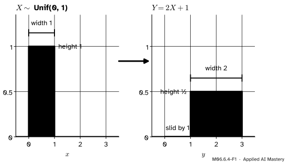
M06.6.4-F1
Doubling and adding 1 sends \({[0, 1]}\) to \({[1, 3]}\). The width doubles, so the height halves: the area, the total probability, stays 1.
Picture the uniform square. Every value of \(X\) in \({[0, 1]}\) becomes \({2X + 1}\) in \({[1, 3]}\), an interval twice as long. The probability that was spread over a length of 1 is now spread over a length of 2, so each unit of length gets half as much: height \({\tfrac12}\).
Build it up
The safe route to a new density is through the CDF (M06.6.3): first find \({\Prob(Y \le y)}\) by turning it into a statement about \(X\), then differentiate.
Step 1. A shift. Let \({Y = X + b}\). Then
\[
\begin{aligned}
F_Y(y) &= \Prob(X + b \le y) \\
&= \Prob(X \le y - b) = F_X(y - b).
\end{aligned}
\]
Differentiate with the chain rule (M04.3.4); the inner function \({y - b}\) has derivative 1, so \({f_Y(y) = f_X(y - b)}\). The graph is the same shape, moved right by \(b\).
Step 2. A stretch. Let \({Y = aX}\) with \({a > 0}\). Dividing both sides of an inequality by a positive number keeps its direction, so
Now the inner function \({y/a}\) has derivative \({1/a}\), and the chain rule brings it out: \({f_Y(y)} = {\tfrac{1}{a} f_X(y/a)}\). The factor \({f_X(y/a)}\) stretches the graph sideways by \(a\); the factor \({1/a}\) lowers it by the same factor.
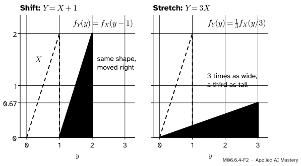
M06.6.4-F2
The hand density \({2x}\) shifted by 1 and stretched by 3. The shift keeps the height; the stretch divides it by 3, from a peak of 2 to a peak of \({\tfrac23}\).
Check the stretch on the hand density with \({a = 3}\): \({f_Y(y) = \tfrac13 \cdot 2\cdot\tfrac{y}{3} =
\tfrac{2y}{9}}\) on \({[0, 3]}\). Its area is \({\int_0^3 \tfrac{2y}{9}\,dy = \tfrac{9}{9} = 1}\). Without the factor \({\tfrac13}\) the area would be 3.
The hook is a stretch: seconds \({S = 60T}\), so \({f_S(s)} = {\tfrac{1}{60} \cdot 0.5\,e^{-0.5 s/60}}\), with peak \({0.5/60}\).
The formal statement
NoteShift and scale
If \(X\) has CDF \({F_X}\) and density \({f_X}\), and \({Y = aX + b}\) with \({a > 0}\), then
Derivation.\({aX + b \le y}\) exactly when \({X \le (y - b)/a}\): subtract \(b\), then divide by the positive \(a\). Take probabilities for the first line. The chain rule, with inner derivative \({1/a}\), gives the second. A negative \(a\) flips the inequality and needs one more step; maps that are not straight lines need more care still. Both wait for M07.1.
A variable \(Z\) with density \({\varphi}\) is written \({Z \sim N(0, 1)}\). For \({\sigma > 0}\), the variable \({X = \mu + \sigma Z}\) is written \({X \sim N(\mu, \sigma^2)}\); by the shift-and-scale rule its density and CDF are
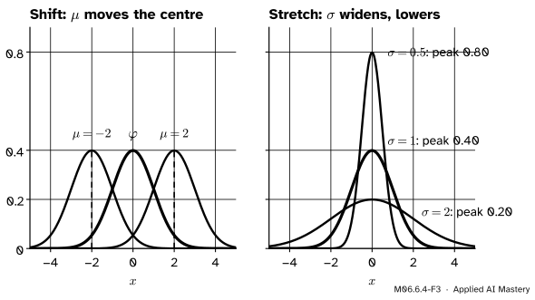
Written out, \({f_X(x)} = {\frac{1}{\sigma\sqrt{2\pi}} e^{-(x - \mu)^2/(2\sigma^2)}}\). The bell is centred on \(\mu\), its peak height is \({\varphi(0)/\sigma} \approx {0.399/\sigma}\), and its spread grows with \({\sigma}\). Module M06.7 shows that \(\mu\) is the mean and \({\sigma^2}\) the variance, which is why the variance is the second parameter.
M06.6.4-F3
The normal family is one shape. \(\mu\) slides it; \(\sigma\) widens it and lowers it by the same factor.
Two facts about \({\varphi}\). First, it is symmetric, \({\varphi(-z) = \varphi(z)}\), so the area left of \({-z}\) equals the area right of \(z\): \({\Phi(-z) = 1 - \Phi(z)}\). Second, its total area is 1. That needs \({\int_{-\infty}^{\infty} e^{-z^2/2}\,dz} = {\sqrt{2\pi}}\), whose proof uses an integral over the plane (M05.6). Here we check it numerically in the code. \({\Phi}\) has no formula in elementary functions; computers use the error function, \({\Phi(z) = \tfrac12\big(1 +
\operatorname{erf}(z/\sqrt{2})\big)}\), available as math.erf.
z-scores. The z-score of a value \(x\) is \({z = (x - \mu)/\sigma}\): how many standard deviations \(x\) sits from \(\mu\). Because \({F_X(x) = \Phi(z)}\), every question about any normal variable becomes a question about \({N(0, 1)}\). Three values are worth knowing:
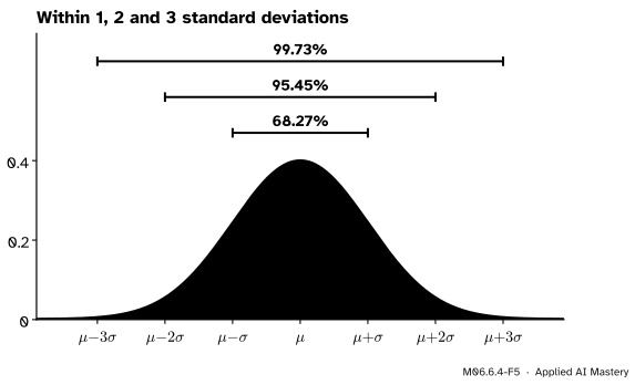
The 68, 95, 99.7 rule: a normal value lands within 1, 2 and 3 standard deviations of its centre about 68%, 95% and 99.7% of the time.
Worked example
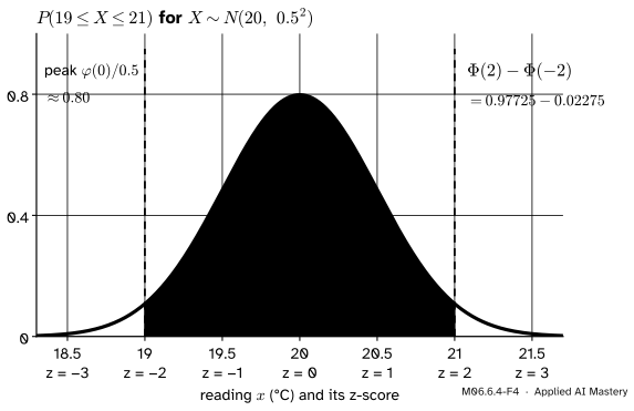
A room thermometer. A thermometer reads the temperature of a room kept at 20 °C, with an error that makes its reading \({X \sim N(20, 0.5^2)}\): \({\mu = 20}\) and \({\sigma = 0.5}\).
Within one degree.\({\Prob(19 \le X \le 21)}\). The z-scores of the two ends are
So the probability is \({\Phi(2) - \Phi(-2)} \approx {0.97725 - 0.02275} = {0.9545}\), as the rule predicts.
A high reading.\({\Prob(X > 21.5)}\): the z-score is \({1.5/0.5 = 3}\), so \({1 - \Phi(3) \approx 0.00135}\), about one reading in 740.
The height of the bell.\({f_X(20)} = {\varphi(0)/0.5} \approx {0.399/0.5} \approx {0.798}\) per degree.
M06.6.4-F4
The thermometer’s reading. Each tick carries its z-score, so 19 to 21 °C is \({-2}\) to 2 on the standard scale, and the shaded area is \({\Phi(2) - \Phi(-2)} \approx {0.9545}\).
Change of units. In Fahrenheit the reading is \({Y = 1.8X + 32}\), a stretch by 1.8 and a shift by 32. Then \({Y} = {1.8(20 + 0.5Z) + 32} = {68 + 0.9Z}\), so \({Y \sim N(68, 0.9^2)}\). Its peak is \({0.798/1.8 \approx 0.443}\) per degree Fahrenheit, lower because a Fahrenheit degree is smaller. Probabilities of matching events do not change: 66.2 °F to 69.8 °F is still 0.9545.
Code
From scratch: \({\varphi}\), \({\Phi}\) from math.erf, a numerical check that the total area of \({\varphi}\) is 1, and the thermometer numbers.
import mathimport numpy as npdef phi(z):return math.exp(-z * z /2) / math.sqrt(2* math.pi)def Phi(z):return0.5* (1+ math.erf(z / math.sqrt(2)))h =0.001# midpoint sum over [-10, 10]area =sum(phi(-10+ (k +0.5) * h) for k inrange(20_000)) * hprint(f"area under phi: {area:.10f}")for k in (1, 2, 3):print(f"P(|Z| <= {k}) = {Phi(k) - Phi(-k):.4f}")mu, sigma =20, 0.5p_within = Phi((21- mu) / sigma) - Phi((19- mu) / sigma)p_high =1- Phi((21.5- mu) / sigma)print(f"P(19 <= X <= 21) = {p_within:.4f}, P(X > 21.5) = {p_high:.5f}")print(f"peak in Celsius {phi(0) / sigma:.3f}, in Fahrenheit {phi(0) / (1.8* sigma):.3f}")
area under phi: 1.0000000000
P(|Z| <= 1) = 0.6827
P(|Z| <= 2) = 0.9545
P(|Z| <= 3) = 0.9973
P(19 <= X <= 21) = 0.9545, P(X > 21.5) = 0.00135
peak in Celsius 0.798, in Fahrenheit 0.443
Now check the shift-and-scale rule on samples: build \({N(20, 0.5^2)}\) from standard normal draws, convert to Fahrenheit, and compare a density-scaled histogram with \({\tfrac{1}{1.8}f_X\big((y -
32)/1.8\big)}\).
rng = np.random.default_rng(4)Z = rng.standard_normal(200_000)X =20+0.5* Z # CelsiusY =1.8* X +32# Fahrenheitheights, edges = np.histogram(Y, bins=12, range=(65.3, 70.7), density=True)mids = (edges[:-1] + edges[1:]) /2rule = np.array([phi(((y -32) /1.8-20) /0.5) /0.5/1.8for y in mids])print("histogram:", np.round(heights, 3))print("rule: ", np.round(rule, 3))print(f"share of X in [19, 21]: {np.mean((X >=19) & (X <=21)):.4f}")
scipy.stats.norm takes loc\({= \mu}\) and scale\({= \sigma}\), the standard deviation.
from scipy import statsreading = stats.norm(loc=20, scale=0.5)print(f"P(19 <= X <= 21) = {reading.cdf(21) - reading.cdf(19):.4f}")print(f"pdf at 20: {reading.pdf(20):.4f} 97.5% quantile of Z: {stats.norm.ppf(0.975):.4f}")
P(19 <= X <= 21) = 0.9545
pdf at 20: 0.7979   97.5% quantile of Z: 1.9600
The 97.5% quantile, about 1.96, is the “2” of the 95% rule made exact: \({\Prob(|Z| \le 1.96) = 0.95}\).
Explore
The module’s interactive is in lesson M06.6.3. Choose the normal density and set \({a = -1}\), \({b = 1}\), then \({-2}\) and 2: the read-out shows 0.6827 and 0.9545, the first two numbers of the rule.
Pitfalls
M06.6.4-F6
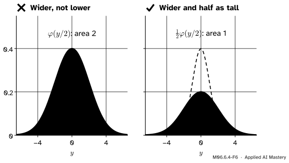
Wrong beside right for \({Y = 2Z}\). Stretching the graph without lowering it doubles the area. The factor \({\tfrac12}\) brings it back to 1.
“To stretch a density by \(a\), replace \(x\) by \({x/a}\).”
That stretches the graph but multiplies its area by \(a\), as the left panel shows. The density must also be divided by \(a\): \({f_Y(y)} = {\tfrac{1}{a} f_X(y/a)}\). Deriving through the CDF, as in Build it up, produces the factor automatically.
“norm(20, 0.25) is \({N(20, 0.5^2)}\), because the variance is 0.25.”
SciPy’s scale is the standard deviation \({\sigma}\), not the variance \({\sigma^2}\). norm(20, 0.25) is half as wide as intended, and norm(loc=20, scale=0.5) is right. The same holds for NumPy’s rng.normal(loc, scale). In machine learning, feature standardisation (subtract the mean, divide by the standard deviation) is the z-score, and dividing by the variance instead is a common slip.
“Real data are normal, so the 68, 95, 99.7 rule always applies.”
The rule is a fact about the normal density only. The waiting time has mean 2 minutes and standard deviation 2 minutes (module M06.8 derives both), so “within one standard deviation of the mean” is 0 to 4 minutes, which holds \({1 - e^{-2} \approx 0.86}\) of the waits, not 0.68. Check the shape before using the rule.
Check yourself
Recall
1. If \({Y = X + b}\), how is \({f_Y}\) related to \({f_X}\)?
Show answer
\({f_Y(y) = f_X(y - b)}\): the same curve moved right by \(b\).
2. If \({Y = aX}\) with \({a > 0}\), how is \({f_Y}\) related to \({f_X}\), and why is there a factor \({1/a}\)?
Show answer
\({f_Y(y)} = {\tfrac{1}{a} f_X(y/a)}\). The same probability is spread over a range \(a\) times as long, so the height must shrink by \(a\) to keep the area 1; the chain rule produces the factor.
3. What is the z-score of \(x\) for \({X \sim N(\mu, \sigma^2)}\), and how does it give \({\Prob(X \le x)}\)?
A normal value lies within 1, 2 and 3 standard deviations of \(\mu\) with probability about 0.68, 0.95 and 0.997.
5. How do you write \({N(20, 0.5^2)}\) in scipy.stats?
Show answer
stats.norm(loc=20, scale=0.5): the scale is the standard deviation.
Exercises
1.★ A test score is \({X \sim N(100, 15^2)}\). Find \({\Prob(X > 130)}\) with the z-score and \({\Phi(2) \approx 0.9772}\).
Show solution
\({z = (130 - 100)/15 = 2}\), so \({\Prob(X > 130)} = {1 - \Phi(2)} \approx {0.0228}\), about one score in 44.
2.★★ The wait \(T\) in minutes has density \({0.5\,e^{-0.5t}}\) for \({t \ge 0}\). Find the density of the wait in seconds, \({S = 60T}\), and its median.
Show solution
With \({a = 60}\): \({f_S(s)} = {\tfrac{1}{60} \cdot 0.5\,e^{-0.5 s/60}} = {\tfrac{1}{120} e^{-s/120}}\) for \({s \ge 0}\), an exponential density with rate \({\tfrac{1}{120}}\) per second. Its median is \({\ln 2 / \tfrac{1}{120}} = {120\ln 2} \approx {83.2}\) seconds, which is 60 times the median of 1.386 minutes, as it must be.
3.★★★ Let \({Y = aX + b}\) with \({a > 0}\). Show directly, by the substitution \({u = (y - b)/a}\), that \({f_Y}\) has total area 1. Then show that the median of \(Y\) is \({a\,m + b}\), where \(m\) is the median of \(X\), and deduce the median of \({N(\mu, \sigma^2)}\).
Show solution
With \({u = (y - b)/a}\), \({du = dy/a}\), and \(u\) runs over the whole line as \(y\) does, so
For the median, \({F_Y(am + b)} = {F_X\big((am + b - b)/a\big)} = {F_X(m)} = {\tfrac12}\). The standard normal has median 0, because \({\varphi}\) is symmetric and so \({\Phi(0) = \tfrac12}\). With \({a = \sigma}\) and \({b = \mu}\), the median of \({N(\mu, \sigma^2)}\) is \({\sigma \cdot 0 + \mu = \mu}\).
Summary card
Shift slides a density; stretch widens it and lowers it.
Standard normal:\({\varphi(z)} = {e^{-z^2/2}/\sqrt{2\pi}}\); \({\Phi(z)} = {\tfrac12(1 + \operatorname{erf}(z/\sqrt2))}\).
\({N(\mu, \sigma^2)}\) is \({\mu + \sigma Z}\), with \({\Prob(X \le x)} = {\Phi\big((x - \mu)/\sigma\big)}\).
68, 95, 99.7 within 1, 2, 3 standard deviations.
SciPy:norm(loc=mu, scale=sigma).
Sources and next steps
Sources. Each was opened and checked against this lesson on 14 November 2026.
Jeremy Orloff and Jonathan Bloom, Reading 5c, Gallery of continuous random variables, MIT OpenCourseWare 18.05, Spring 2022: the normal density and the rule of thumb \({\Prob(|Z| \le 1)} \approx {0.68}\), \({\Prob(|Z| \le 2)} \approx {0.95}\), \({\Prob(|Z| \le 3)} \approx {0.99}\), with exact values from software. Reading 5d, Manipulating continuous random variables, Section 2.1: transform the CDF first, step by step from its definition, then differentiate.
Hossein Pishro-Nik, Section 4.2.3, Normal (Gaussian) distribution: the standard normal density \({\frac{1}{\sqrt{2\pi}}e^{-z^2/2}}\), \({\Phi}\) as its integral with no closed form, \({X = \sigma Z + \mu}\) as \({N(\mu, \sigma^2)}\), and \({F_X(x)} = {\Phi\big((x - \mu)/\sigma\big)}\).
Charles M. Grinstead and J. Laurie Snell, Introduction to Probability, Section 5.2: Theorem 5.1 gives \({F_Y(y)} = {F_X(\varphi^{-1}(y))}\) for a strictly increasing \({\varphi}\), and Corollary 5.1 the matching density by the chain rule.
SciPy reference, scipy.stats.norm: loc is the mean and scale the standard deviation, and norm.pdf(x, loc, scale) equals norm.pdf(y) / scale with \({y} = {(x - \text{loc})/\text{scale}}\), the shift-and-scale rule.
Next. Module M06.7 turns the balance point and the spread of a density into numbers, the expectation and the variance, and shows that \(\mu\) and \({\sigma^2}\) are exactly those. The normal bell returns in M06.11 as the shape that averages settle on.