The CDF of a continuous variable is the area under its density to the left of x, and its slope is the density. Read medians and other quantiles off it, then turn it round to make any distribution out of uniform random numbers.
M06.6.3L1 Core25 minIn review (what this means)
The maths and code on this page are checked by automated tests on every change, but an independent reader has not signed it off yet. Spot a mistake or a confusing step? Tell us.
Find the CDF of a continuous variable as the area to the left of x, and recover the density as its derivative.
Compute P(a < X ≤ b) as F(b) − F(a) and read the same number off a graph of F.
Find quantiles by inverting the CDF: the median of 2x is 1/√2 and the median wait is ln 2 / λ.
Derive inverse-CDF sampling and use it to draw from the density 2x and from an exponential, from scratch and with scipy.stats.
The question
A computer’s random number generator makes one kind of randomness: numbers spread evenly between 0 and 1. Yet NumPy hands out waiting times, normal values and dart distances on demand, and a language model draws its next word from whatever distribution it has learned. How do you turn an even spread into any spread you like? The answer comes from one curve, the CDF, read backwards.
From the last lesson
1. For which constant \(c\) is \({cx}\) on \({[0, 1]}\) a density?
Show answer
\({c = 2}\), because \({\int_0^1 cx\,dx = c/2}\) must be 1.
2. For a waiting time with density \({\lambda e^{-\lambda t}}\), what is \({\Prob(T > t)}\)?
Show answer
\({e^{-\lambda t}}\). With \({\lambda = 0.5}\) and \({t = 4}\) that is \({e^{-2} \approx 0.135}\).
Intuition
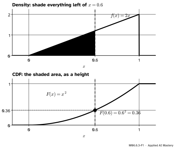
In module M06.5 the cumulative distribution function of a discrete variable was a staircase, \({F(x) = \Prob(X \le x)}\), jumping at each value. The definition carries over word for word. For a continuous variable, \({\Prob(X \le x)}\) is the area under the density to the left of \(x\).
M06.6.3-F1
The CDF turns an area into a height. Above, the area under \({2x}\) left of 0.6 is 0.36. Below, the CDF \({F(x) = x^2}\) passes through height 0.36 at \({x = 0.6}\).
Slide the orange line from left to right. The shaded area can only grow, from 0 far to the left to 1 far to the right, and it grows fastest where the density is tallest. Where the density is 0 nothing is added, and the CDF is flat. So the CDF is a smooth ramp instead of a staircase, steep where values are common.
Build it up
Step 1. The CDF of the hand density. For \({0 \le x \le 1}\),
To the left of 0 no area has been gathered, so \({F(x) = 0}\); to the right of 1 all of it has, so \({F(x) = 1}\). (The letter \(s\) inside the integral is a dummy name; \(x\) is busy as the upper limit.)
Step 2. The slope of the CDF is the density. By part one of the fundamental theorem (M04.6.2), the area up to \(x\) grows at the rate of the height at \(x\):
\[
F'(x) = f(x)
\]
at every \(x\) where \(f\) is continuous.
Check: \({\frac{d}{dx}x^2 = 2x}\). So either one gives the other: integrate the density to get the CDF, differentiate the CDF to get the density.
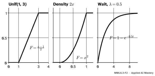
Step 3. The other two running densities. For \({\text{Unif}(a, b)}\) the area to the left of \(x\) in \({[a, b]}\) is a rectangle, so \({F(x) = (x - a)/(b - a)}\). For the waiting time, \({F(t)}\) is 1 minus the tail of M06.6.2, so \({F(t) = 1 - e^{-\lambda t}}\) for \({t \ge 0}\).
M06.6.3-F2
Three CDFs. Each climbs from 0 to 1 and never falls; each is steepest where its density is tallest.
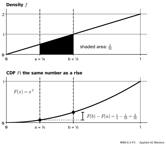
Step 4. Intervals from the CDF. The area left of \(b\) is the area left of \(a\) plus the area between them. Rearranged:
\[
\Prob(a < X \le b) = F(b) - F(a).
\]
For a continuous variable the end points do not matter (M06.6.1), so this is also \({\Prob(a \le X \le b)}\).
M06.6.3-F3
One number, two pictures: the area between \(a\) and \(b\) under the density is the rise of the CDF from \(a\) to \(b\).
With \({a = \tfrac14}\) and \({b = \tfrac12}\) this gives \({\tfrac14 - \tfrac{1}{16}} = {\tfrac{3}{16}}\), the answer of M06.6.2 read straight off the CDF.
The formal statement
NoteDefinitions: CDF, quantile function
The CDF of a random variable \(X\) with density \(f\) is
It never falls, it tends to 0 as \({x \to -\infty}\) and to 1 as \({x \to \infty}\), \({F'(x) = f(x)}\) wherever \(f\) is continuous, and \({\Prob(a < X \le b)} = {F(b) - F(a)}\).
When \(F\) is continuous and strictly increasing on the range of \(X\), the quantile function is its inverse: for \({0 < p < 1}\), \({Q(p)}\) is the one \(x\) with \({F(x) = p}\). The median is \({Q(\tfrac12)}\).
\({Q(p)}\) is the value that a share \(p\) of the probability lies below. The median splits the area under the density into two halves; \({Q(0.25)}\) and \({Q(0.75)}\), the quartiles, split it into quarters.
Inverse-CDF sampling. Let \({U \sim \text{Unif}(0, 1)}\) and set \({X = Q(U)}\). Then \(X\) has CDF \(F\).
Proof. Fix \(x\) in the range. Because \(F\) is strictly increasing there, the two inequalities \({Q(u) \le x}\) and \({u \le F(x)}\) say the same thing: apply \(F\) to both sides of the first, or \(Q\) to both sides of the second. So the events \({\{Q(U) \le x\}}\) and \({\{U \le F(x)\}}\) are equal, and
The last step holds because \({\Prob(U \le p) = p}\) for a uniform \(U\) and any \(p\) in \({[0, 1]}\). ∎
M06.6.3-F5
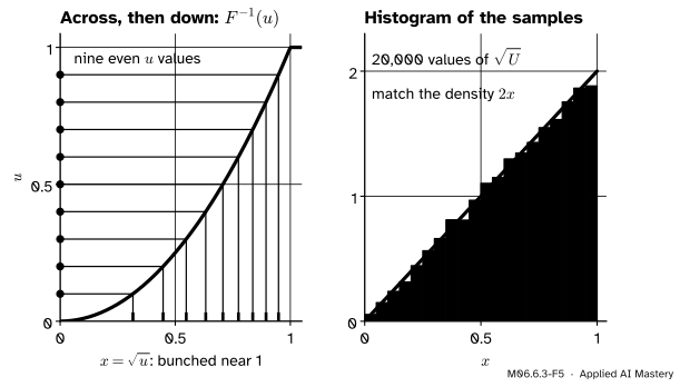
Inverse-CDF sampling for the density \({2x}\). Left: evenly spaced heights \(u\), sent across to the CDF and down, land bunched where the CDF is steep. Right: 20,000 values of \({\sqrt{U}}\) fill in the density \({2x}\).
The left panel shows why it works. Equal steps in \(u\) are equal shares of probability. Where the CDF is steep, an equal share is covered by a short stretch of \(x\), so the samples crowd together exactly where the density is tall.
Worked example
Medians, and a few samples.
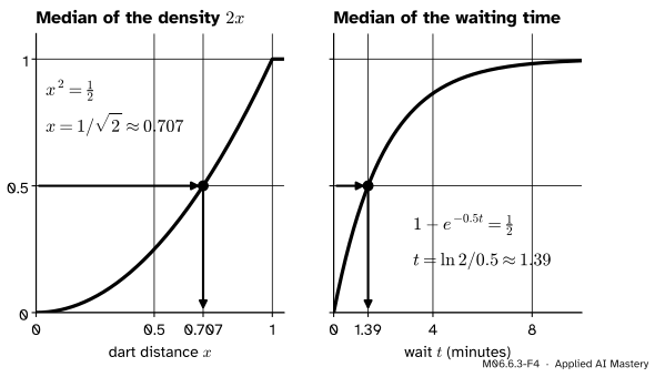
The hand density. Solve \({F(x) = \tfrac12}\) on \({[0, 1]}\): \({x^2 = \tfrac12}\), so the median is \({x = 1/\sqrt{2} \approx 0.707}\). Half the darts land beyond 0.707 of the radius. In general \({Q(p) = \sqrt{p}}\), so the quartiles are \({\sqrt{0.25} = 0.5}\) and \({\sqrt{0.75} \approx 0.866}\).
The waiting time. Solve \({1 - e^{-\lambda t} = p}\) step by step:
\[
\begin{aligned}
e^{-\lambda t} &= 1 - p \\
-\lambda t &= \ln(1 - p) \\
t &= -\ln(1 - p)/\lambda .
\end{aligned}
\]
With \({p = \tfrac12}\), \({-\ln \tfrac12 = \ln 2}\), so the median wait is \({\ln 2/\lambda}\). For \({\lambda = 0.5}\) that is \({2\ln 2 \approx 1.386}\) minutes. Half of all waits are over in under 1.39 minutes, although the average wait quoted in M06.6.2 was 2 minutes; the long tail pulls the mean above the median.
M06.6.3-F4
Reading a quantile: across from the height \(p\) to the CDF, then down. For \({p = \tfrac12}\) this gives the median, 0.707 for the dart and 1.39 minutes for the wait.
Five samples by hand. Take five uniform numbers, \({u} = {0.04, 0.25, 0.49, 0.64, 0.81}\), and apply \({Q(u) = \sqrt{u}}\). The dart distances are \({0.2, 0.5, 0.7, 0.8, 0.9}\). The same five numbers sent through the waiting-time quantile \({-2\ln(1 - u)}\) give waits of about 0.08, 0.58, 1.35, 2.04 and 3.32 minutes.
Code
From scratch: the CDF, the quantile function and the sampler for the hand density, then a histogram check.
import mathimport numpy as npdef F_hand(x):returnmin(max(x, 0.0), 1.0) **2def Q_hand(p):return math.sqrt(p)def Q_wait(p, lam=0.5):return-math.log(1- p) / lamprint("F(0.6) =", round(F_hand(0.6), 4), " P(1/4 < X <= 1/2) =", F_hand(0.5) - F_hand(0.25))print("median of 2x:", round(Q_hand(0.5), 4), " quartiles:", Q_hand(0.25), round(Q_hand(0.75), 4))print("median wait:", round(Q_wait(0.5), 4), "minutes")u = [0.04, 0.25, 0.49, 0.64, 0.81]print("darts:", [round(Q_hand(p), 2) for p in u])print("waits:", [round(Q_wait(p), 2) for p in u])
F(0.6) = 0.36   P(1/4 < X <= 1/2) = 0.1875
median of 2x: 0.7071   quartiles: 0.5 0.866
median wait: 1.3863 minutes
darts: [0.2, 0.5, 0.7, 0.8, 0.9]
waits: [0.08, 0.58, 1.35, 2.04, 3.32]
Now many samples at once, with NumPy doing the square roots and logarithms for a whole array.
rng = np.random.default_rng(6)U = rng.uniform(size=200_000)darts = np.sqrt(U) # density 2xwaits =-np.log(1- U) /0.5# rate 0.5heights, edges = np.histogram(darts, bins=10, range=(0, 1), density=True)mids = (edges[:-1] + edges[1:]) /2print("dart histogram:", np.round(heights, 2))print("2x at midpoints:", np.round(2* mids, 2))print(f"share of darts below 0.707: {np.mean(darts <=1/ math.sqrt(2)):.4f}")print(f"median of the simulated waits: {np.median(waits):.3f}")
dart histogram: [0.1  0.29 0.5  0.71 0.9  1.1  1.29 1.51 1.7  1.9 ]
2x at midpoints: [0.1 0.3 0.5 0.7 0.9 1.1 1.3 1.5 1.7 1.9]
share of darts below 0.707: 0.4995
median of the simulated waits: 1.388
scipy.stats packages every distribution with its cdf and its quantile function, which it calls ppf (percent point function). The exponential takes scale\({= 1/\lambda}\), the uniform on \({[a, b]}\) takes loc=a, scale=b - a, and the density \({2x}\) is the family that SciPy calls beta(2, 1), met in later courses.
from scipy import statswait = stats.expon(scale=1/0.5)print(f"P(T <= 4) = {wait.cdf(4):.4f}, median = {wait.ppf(0.5):.4f}")bus = stats.uniform(loc=2, scale=4) # Unif(2, 6)print(f"bus: P(3 <= X <= 4.5) = {bus.cdf(4.5) - bus.cdf(3):.3f}")hand = stats.beta(2, 1) # density 2x on [0, 1]print(f"hand: F(0.6) = {hand.cdf(0.6):.2f}, median = {hand.ppf(0.5):.4f}")print("sampler:", np.round(wait.ppf(np.array(u)), 2))
P(T <= 4) = 0.8647, median = 1.3863
bus: P(3 <= X <= 4.5) = 0.375
hand: F(0.6) = 0.36, median = 0.7071
sampler: [0.08 0.58 1.35 2.04 3.32]
SciPy’s ppf applied to uniform numbers is the same sampler: wait.ppf(U) and the hand-made -np.log(1 - U) / 0.5 are the same function.
Explore
M06.6-X1
Area under a density
Choose a density and drag the two orange handles, or use the sliders, to set \(a\) and \(b\). The shaded area above and the rise of the CDF below always show the same number. Press Squeeze again and again: the interval closes in on one value, the probability falls to 0, and the height of the density does not move.
Pitfalls
M06.6.3-F6
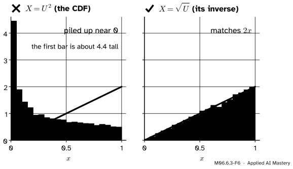
Wrong beside right. Pushing uniform numbers through the CDF \({x^2}\) piles them up near 0. Pushing them through its inverse \({\sqrt{u}}\) gives the density \({2x}\).
“To sample from \({F(x) = x^2}\), square a uniform number.”
Squaring sends \(u\) to \({F(u)}\), the wrong direction. A sample is the \(x\) whose CDF value is \(u\), so solve \({x^2 = u}\): \({x = \sqrt{u}}\). In words: go across from \(u\) on the vertical axis to the curve, then down. Starting on the horizontal axis and going up is the CDF, not the sampler.
“The median is where the density is highest, or halfway along the range.”
The density \({2x}\) is highest at 1, and the middle of its range is 0.5, but its median is 0.707. The median splits the area in half. For the waiting time the density is highest at 0 and the median is 1.39 minutes.
“The CDF at \(x\) is the chance of \(x\).”
\({F(0.6) = 0.36}\) is the chance of a value at most 0.6, the whole area to the left. The chance of exactly 0.6 is 0, and the density there, 1.2, is a rate, not a chance.
Check yourself
Recall
1. What is the CDF of the hand density \({2x}\) on \({[0, 1]}\), and what is it to the left of 0 and to the right of 1?
Show answer
\({F(x) = x^2}\) on \({[0, 1]}\); it is 0 to the left of 0 and 1 to the right of 1.
2. How do you get the density back from the CDF?
Show answer
Differentiate: \({f(x) = F'(x)}\) wherever \(f\) is continuous (the fundamental theorem).
3. Write \({\Prob(a < X \le b)}\) in terms of the CDF.
Show answer
\({F(b) - F(a)}\).
4. What is the median wait when \({\lambda = 0.5}\) per minute?
2.★★ A variable has CDF \({F(x) = x^3}\) on \({[0, 1]}\). Find its density, its median, and a formula that turns a uniform number \(u\) into a sample.
Show solution
The density is \({F'(x) = 3x^2}\) on \({[0, 1]}\). The median solves \({x^3 = \tfrac12}\), so \({x = 2^{-1/3} \approx 0.794}\). Solving \({x^3 = u}\) gives the sampler \({x = u^{1/3}}\).
3.★★★ Show that if \(X\) has a continuous, strictly increasing CDF \(F\), then \({U = F(X)}\) is uniform on \({[0, 1]}\): the inverse-CDF method run backwards. Check it for the hand density.
Show solution
For \({0 \le u \le 1}\), the events \({\{F(X) \le u\}}\) and \({\{X \le Q(u)\}}\) are equal, because \(F\) and \(Q\) are increasing inverses of each other. So
which is the CDF of \({\text{Unif}(0, 1)}\). For the hand density, \({U = X^2}\) and \({\Prob(X^2 \le u)} = {\Prob(X \le \sqrt{u})} = {(\sqrt{u})^2} = {u}\). This result is called the probability integral transform.
Intervals:\({\Prob(a < X \le b)} = {F(b) - F(a)}\).
Quantile:\({Q(p)}\) solves \({F(x) = p}\); median of \({2x}\) is \({1/\sqrt{2}}\), median wait \({\ln 2/\lambda}\).
Sampling:\({X = Q(U)}\) has CDF \(F\): \({\sqrt{U}}\) has density \({2x}\).
In SciPy:cdf and ppf, with expon(scale=1/lam).
Sources and next steps
Sources. Each was opened and checked against this lesson on 14 November 2026.
Jeremy Orloff and Jonathan Bloom, Reading 5b, Continuous random variables, MIT OpenCourseWare 18.05, Spring 2022. Section 4.3 defines the CDF as an integral of the density (Example 6: \({3x^2}\) has CDF \({x^3}\)); Section 4.4 lists its properties, including \({\Prob(a \le X \le b)} = {F(b) - F(a)}\) and \({F' = f}\) by the fundamental theorem.
Charles M. Grinstead and J. Laurie Snell, Introduction to Probability, Section 5.2. Theorem 5.1 relates the CDF of \({\varphi(X)}\) to that of \(X\) for an increasing \({\varphi}\), and Corollary 5.2 states that \({F^{-1}(U)}\) has CDF \(F\) when \(U\) is uniform on \({[0, 1]}\), the basis of simulation.
Marc Peter Deisenroth, A. Aldo Faisal and Cheng Soon Ong, Mathematics for Machine Learning, Section 6.2.2 (Definition 6.2, the CDF as an integral of the density) and Section 6.7.1 (Theorem 6.15, the probability integral transform, and its use for sampling by the inverse CDF).
SciPy reference, scipy.stats.expon: the rate form \({\lambda e^{-\lambda x}}\) corresponds to scale = 1/λ; ppf is the inverse of cdf.