Check that a function is a density, find the constant that makes it one, and compute probabilities by integrating: for the uniform, the density 2x and a waiting time whose tail runs to infinity, then with a Riemann sum and scipy.integrate.quad.
M06.6.2L1 Core25 minIn review (what this means)
The maths and code on this page are checked by automated tests on every change, but an independent reader has not signed it off yet. Spot a mistake or a confusing step? Tell us.
Check that a function is a density and find the constant that makes a function into one.
Compute interval probabilities for Unif(a, b) and for the density 2x by integrating by hand.
Derive the tail P(T > t) = e^(-λt) of an exponential waiting time as a limit of integrals.
Approximate a probability with a Riemann sum written from scratch and confirm it with scipy.integrate.quad.
The question
Requests reach a web server at random, on average one every 2 minutes. A common model for the wait \(T\) until the next one is the density \({f(t) = 0.5\,e^{-0.5t}}\) for \({t \ge 0}\). What is the chance of waiting more than 4 minutes? The answer is an area under a curve that never reaches zero, so the area runs on for ever. How do you compute it, and how do you know the formula was a density at all?
From the last lesson
1. Can a density be larger than 1? Give an example.
Show answer
Yes. \({\text{Unif}(0, 0.5)}\) has height 2 on \({[0, 0.5]}\), and its total area is still 1.
2. How do you turn the count in a histogram bar into a density height?
Show answer
Divide the count by the number of samples to get a share, then divide the share by the bin width.
Intuition
Lesson M06.6.1 found that for a continuous random variable every probability is an area under the density. Computing a probability is therefore computing an integral, and the tools of M04.5 to M04.7 do all the work: an antiderivative when there is one, a limit when the range is infinite, a Riemann sum when nothing else will do.
M06.6.2-F1
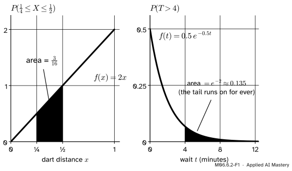
Two probabilities as areas. Left: the dart distance of M06.6.1 lands between \({\tfrac14}\) and \({\tfrac12}\) with probability \({\tfrac{3}{16}}\). Right: the wait is longer than 4 minutes with probability \({e^{-2} \approx 0.135}\), the area of a tail with no right-hand end.
The left panel uses this course’s hand density, \({f(x) = 2x}\) on \({[0, 1]}\): the dart distance, small enough to work entirely by hand. The right panel uses the waiting time with rate \({\lambda = 0.5}\) per minute. Both are running examples from here to the end of the course.
Build it up
Step 1. Checking a density. A proposed density must pass the two tests of M06.6.1. It must never be negative, and its total area must be 1. The second test is an integral. For \({2x}\) on \({[0, 1]}\):
It is never negative on \({[0, 1]}\), and it is 0 elsewhere, so it passes.
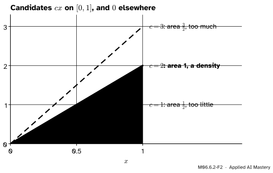
Step 2. Finding the constant. Often the shape of a density is known and only its size is missing. Suppose the chance of a value near \(x\) should grow in proportion to \(x\) on \({[0, 1]}\). Then \({f(x) = cx}\) for some constant \({c > 0}\). The area must be 1:
so \({c = 2}\). The constant that makes the area 1 is called the normalising constant.
M06.6.2-F2
Only one member of the family \({cx}\) encloses area 1. Too small a constant leaves probability missing; too large a constant creates more than there is.
The same step works for the waiting time. If the density has the shape \({e^{-0.5t}}\) for \({t \ge 0}\), then \({f(t) = c\,e^{-0.5t}}\), and the area out to infinity must be 1. Step 4 shows that \({\int_0^\infty e^{-0.5t}\,dt} = {2}\), so \({c = 0.5}\).
Step 3. Probabilities are integrals over intervals. With the density in hand, any probability about \(X\) is an integral, and the fundamental theorem (M04.6.3) evaluates it from an antiderivative.
Step 4. A range with no end. The area under \({f(t)} = {\lambda e^{-\lambda t}}\) cannot be shaded all at once, because the curve runs on for ever. As in M04.7.3, shade it up to a finite end \(M\) and let \(M\) grow. An antiderivative of \({\lambda e^{-\lambda t}}\) is \({-e^{-\lambda t}}\) (differentiate it to check: the chain rule brings down \({-\lambda}\)). So
As \({M \to \infty}\), \({e^{-\lambda M} \to 0}\) for any \({\lambda > 0}\), so the total area is 1: the waiting-time density passes the test.
The formal statement
NoteThree densities and their probabilities
Uniform, \({X \sim \text{Unif}(a, b)}\) with \({a < b}\): \({f(x) = \frac{1}{b - a}}\) on \({[a, b]}\), and 0 elsewhere. For \({a \le c \le d \le b}\),
\[
\Prob(c \le X \le d) = \frac{d - c}{b - a}.
\]
Hand density, \({f(x) = 2x}\) on \({[0, 1]}\): for \({0 \le c \le d \le 1}\), \({\Prob(c \le X \le d)} = {d^2 - c^2}\).
Exponential, \({T \sim \text{Exp}(\lambda)}\) with rate \({\lambda > 0}\): \({f(t)} = {\lambda e^{-\lambda t}}\) for \({t \ge 0}\), and 0 for \({t < 0}\). For \({t \ge 0}\),
\[
\Prob(T > t) = e^{-\lambda t}.
\]
Uniform. The density is a flat line, so the area over \({[c, d]}\) is a rectangle of width \({d - c}\) and height \({1/(b - a)}\). With the integral: \({\int_c^d \frac{dx}{b - a}} = {\frac{d - c}{b - a}}\). Over the whole of \({[a, b]}\) this is 1.
Hand density. An antiderivative of \({2x}\) is \({x^2}\), so \({\int_c^d 2x\,dx = d^2 - c^2}\). For instance, \({\Prob(X \le \tfrac12)} = {\tfrac14 - 0} = {\tfrac14}\): the inner half of the distances holds only a quarter of the darts.
Exponential tail. The event \({T > t}\) is an interval with no right-hand end, so its probability is the limit of the areas from \(t\) to \(M\):
The middle line uses the antiderivative of Step 4: \({-e^{-\lambda M} - (-e^{-\lambda t})}\).
M06.6.2-F4
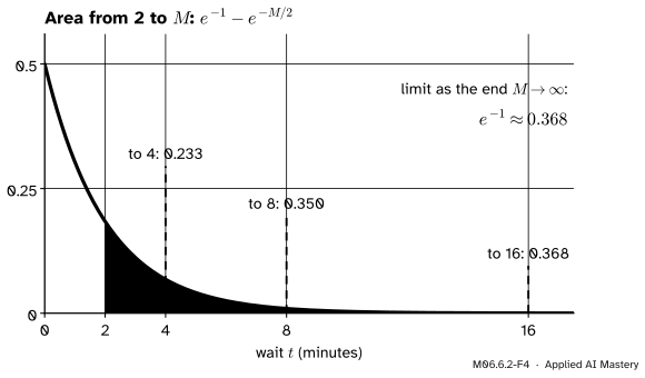
The tail beyond 2 minutes, built up by moving the right end out. The areas 0.233, 0.350 and 0.368 close in on \({e^{-1} \approx 0.368}\).
With \({\lambda = 0.5}\) the tail gives \({\Prob(T > 2)} = {e^{-1}} \approx {0.368}\) and \({\Prob(T > 4)} = {e^{-2}} \approx {0.135}\), which answers the question: about one wait in seven lasts more than 4 minutes. An interval in the middle is a difference of two tails, because \({\{T > 1\}}\) is \({\{1 < T \le 3\}}\) together with \({\{T > 3\}}\):
Split each minute into \(n\) short slots and suppose a request arrives in each slot with chance \({\lambda/n}\), independently. Waiting more than \(t\) minutes means \({nt}\) empty slots in a row, with chance \({(1 - \lambda/n)^{nt}}\). As \({n \to \infty}\) this tends to \({e^{-\lambda t}}\), the tail above. Module M06.8 derives this limit and proves that such waits are memoryless.
Worked example
Find \({\Prob(\tfrac14 \le X \le \tfrac12)}\) for the hand density \({2x}\), three ways.
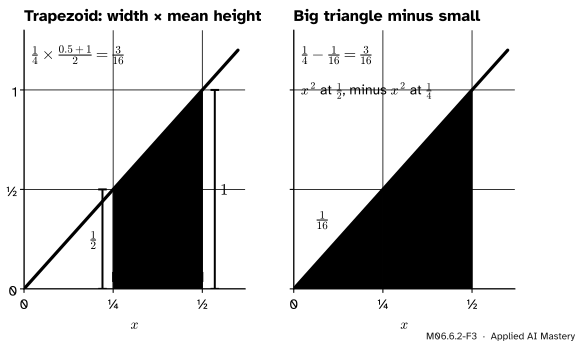
As a trapezoid. The region is a trapezoid of width \({\tfrac14}\), with heights \({2 \cdot \tfrac14 =
\tfrac12}\) and \({2 \cdot \tfrac12 = 1}\) at its two sides. Its area is the width times the mean height: \({\tfrac14 \times \tfrac{1}{2}(\tfrac12 + 1)} = {\tfrac14 \times \tfrac34} = {\tfrac{3}{16}}\).
As a difference of triangles. The triangle under \({2x}\) from 0 to \({\tfrac12}\) has area \({\tfrac12 \times \tfrac12 \times 1} = {\tfrac14}\); the one from 0 to \({\tfrac14}\) has area \({\tfrac12 \times \tfrac14 \times \tfrac12} = {\tfrac{1}{16}}\). Take one from the other.
M06.6.2-F3
The same \({\tfrac{3}{16}}\) two more ways. The difference of triangles is exactly what the antiderivative \({x^2}\) computes.
All three agree, and the third shows what the antiderivative is: \({x^2}\) is the area from 0 up to \(x\). Lesson M06.6.3 gives that area a name. By the complement rule (M06.1.4), the chance that a dart lands in the outer half of the radius is \({\Prob(X > \tfrac12)} = {1 - \tfrac14} = {\tfrac34}\).
Code
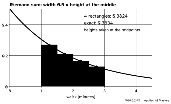
A Riemann sum (M04.5.2) needs no antiderivative: cut the interval into \(n\) strips, take the density at the middle of each, and add up height times width. From scratch, for \({\Prob(1 \le T \le 3)}\):
import mathlam =0.5def f_wait(t):"""The waiting-time density: lam * e^(-lam t) for t >= 0, and 0 before."""return lam * math.exp(-lam * t) if t >=0else0.0def midpoint_sum(f, a, b, n):"""Area under f from a to b, from n strips with heights taken at their midpoints.""" h = (b - a) / nreturnsum(f(a + (k +0.5) * h) for k inrange(n)) * hexact = math.exp(-0.5) - math.exp(-1.5)for n in (4, 10, 100, 1000): approx = midpoint_sum(f_wait, 1, 3, n)print(f"n = {n:4d}: {approx:.6f} error {approx - exact:+.1e}")print(f"exact: {exact:.6f}")
n =    4: 0.382404   error -1.0e-03
n =   10: 0.383241   error -1.6e-04
n =  100: 0.383399   error -1.6e-06
n = 1000: 0.383400   error -1.6e-08
exact:      0.383400
M06.6.2-F5
Four rectangles already give 0.3824 against the exact 0.3834. Each rectangle gains a little on one side of its midpoint and loses a little on the other.
The error shrinks a hundredfold each time \(n\) grows tenfold, the rate the midpoint rule promises. scipy.integrate.quad does the same job adaptively, and it accepts np.inf as a limit, so a tail needs no hand-made limit.
import numpy as npfrom scipy.integrate import quadtotal, _ = quad(f_wait, 0, np.inf)tail_4, _ = quad(f_wait, 4, np.inf)middle, _ = quad(f_wait, 1, 3)dart, _ = quad(lambda x: 2* x, 0.25, 0.5)print(f"total area {total:.6f}, P(T > 4) = {tail_4:.4f}, P(1 <= T <= 3) = {middle:.4f}")print(f"P(1/4 <= X <= 1/2) = {dart:.6f} (3/16 = {3/16})")rng = np.random.default_rng(1)waits = rng.exponential(scale=1/ lam, size=200_000) # NumPy takes the scale 1/lam, not the rateprint(f"simulated share of waits above 4: {np.mean(waits >4):.4f}")
total area 1.000000, P(T > 4) = 0.1353, P(1 <= T <= 3) = 0.3834
P(1/4 <= X <= 1/2) = 0.187500  (3/16 = 0.1875)
simulated share of waits above 4: 0.1338
The integrals agree with the hand results, and 200,000 simulated waits give a share above 4 minutes close to \({e^{-2} \approx 0.1353}\).
Explore
The interactive of this module is in lesson M06.6.3. Choose the exponential density, set \({a = 4}\) and drag \(b\) to the far right: the area climbs to 0.1286, close to the tail \({e^{-2} \approx 0.1353}\); the rest lies beyond the edge of the drawing.
Pitfalls
M06.6.2-F6
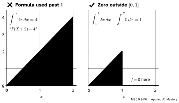
Wrong beside right. The formula \({2x}\) holds only on \({[0, 1]}\). Beyond 1 the density is 0, so \({\Prob(X \le 2) = 1}\), not 4.
“The density is \({2x}\), so \({\Prob(X \le 2)} = {\int_0^2 2x\,dx} = {4}\).”
A density formula comes with a range, and outside it the density is 0. Split the integral where the formula changes: \({\int_0^1 2x\,dx + \int_1^2 0\,dx} = {1}\). A probability above 1 is always a sign that a range has been forgotten.
“rng.exponential(0.5) draws waits with rate 0.5.”
NumPy’s exponential and SciPy’s expon take the scale\({1/\lambda}\), which is the mean wait, not the rate. rng.exponential(0.5) draws waits with mean 0.5 minutes, four times too short for this lesson’s \({\lambda = 0.5}\). Write scale=1 / lam and the mistake cannot happen.
“The constant does not matter; only the shape does.”
The shape fixes which values are more likely, but probabilities need the constant. Fitting a model by its likelihood in machine learning relies on the density having area 1; a model that could raise its density everywhere would score better without fitting anything. Normalising is what stops it.
Check yourself
Recall
1. What two things do you check to decide whether a function is a density?
Show answer
That it is never negative, and that its total area (its integral over the whole line) is 1.
2. For which constant \(c\) is \({cx}\) on \({[0, 1]}\) a density?
Show answer
\({c = 2}\), because \({\int_0^1 cx\,dx = c/2}\) must be 1.
3. If \({X \sim \text{Unif}(a, b)}\), what is \({\Prob(c \le X \le d)}\) for \({a \le c \le d \le b}\)?
Show answer
\({(d - c)/(b - a)}\): the length of the interval over the length of the range.
4. For a waiting time with density \({\lambda e^{-\lambda t}}\), what is \({\Prob(T > t)}\)?
Show answer
\({e^{-\lambda t}}\). With \({\lambda = 0.5}\) and \({t = 4}\) that is \({e^{-2} \approx 0.135}\).
5. Why is an integral out to infinity written as a limit?
Show answer
An area with no right-hand end cannot be computed in one go. It is defined as the limit of the areas up to a finite end \(M\) as \({M \to \infty}\), when that limit exists (M04.7.3).
Exercises
1.★ A bus arrives at a random time, uniformly between 2 and 6 minutes from now. Find the chance that it arrives between 3 and 4.5 minutes from now.
Show solution
\({X \sim \text{Unif}(2, 6)}\) has density \({\tfrac14}\) on \({[2, 6]}\), so \({\Prob(3 \le X \le 4.5)} = {(4.5 - 3)/(6 - 2)} = {1.5/4} = {0.375}\).
2.★★ A density has the form \({f(x) = cx^2}\) on \({[0, 3]}\), and 0 elsewhere. Find \(c\), then \({\Prob(X \le 1.5)}\).
Show solution
The area is \({\int_0^3 cx^2\,dx} = {c\big[\tfrac{x^3}{3}\big]_0^3} = {9c}\), so \({c = \tfrac19}\). Then
Half the range holds only an eighth of the probability, because the density grows like \({x^2}\).
3.★★★ For the waiting time with \({\lambda = 0.5}\), find the time \(t\) that only 5% of waits exceed. Then show that \({\Prob(T > 2t)} = {\Prob(T > t)^2}\) for every \({t \ge 0}\), and say what it means in words.
Show solution
Solve \({e^{-0.5t} = 0.05}\). Take logarithms: \({-0.5t = \ln 0.05 = -\ln 20}\), so \({t = 2\ln 20 \approx 5.99}\) minutes. For the second part, \({\Prob(T > 2t)} = {e^{-2\lambda t}} = {(e^{-\lambda t})^2} = {\Prob(T > t)^2}\). In words: surviving \({2t}\) minutes without a request is like surviving \(t\) minutes twice in a row, independently, which is the memoryless property that module M06.8 proves.
Summary card
A probability is an integral of the density.
M06.6.2-F1
A bounded interval, and a tail.
Check a density:\({f \ge 0}\) and \({\int f = 1}\); solve the second for a missing constant.
Hand density \({2x}\):\({\Prob(c \le X \le d)} = {d^2 - c^2}\), so \({\Prob(\tfrac14 \le X \le \tfrac12)} = {\tfrac{3}{16}}\).
Exponential:\({\Prob(T > t)} = {e^{-\lambda t}}\), a limit of integrals.
Numerically: a midpoint sum from scratch, then scipy.integrate.quad, which accepts np.inf.
Sources and next steps
Sources. Each was opened and checked against this lesson on 14 November 2026.
Jeremy Orloff and Jonathan Bloom, Reading 5b, Continuous random variables, MIT OpenCourseWare 18.05, Spring 2022. Section 4.2 works probabilities as areas (Example 2, a density of height 3), finds a normalising constant (Example 3, \({Cx^2}\) on \({[0, 1]}\) gives \({C = 3}\)) and integrates for a probability (Example 4).
Hossein Pishro-Nik, Section 4.1.1 finds the constant \(c\) in \({c\,e^{-x}}\) by integrating and computes \({\Prob(1 < X < 3)}\); and Section 4.2.2 gives the exponential density \({\lambda e^{-\lambda x}}\) for \({x \ge 0}\), its CDF \({1 - e^{-\lambda x}}\) and its mean \({1/\lambda}\).
Charles M. Grinstead and J. Laurie Snell, Introduction to Probability, Section 2.2, Example 2.12: the dart-distance density \({2r}\) and \({\Prob([a, b]) = b^2 - a^2}\).
SciPy reference, scipy.integrate.quad: returns the integral and an estimate of its absolute error, and takes numpy.inf for an infinite limit.