A spinner that can stop anywhere gives every single value probability 0, yet intervals still have probabilities. Scale a histogram so that area is probability, narrow its bins, and the bars settle on a curve: the density.
M06.6.1L1 Core25 minIn review (what this means)
The maths and code on this page are checked by automated tests on every change, but an independent reader has not signed it off yet. Spot a mistake or a confusing step? Tell us.
Explain why a spinner that can stop anywhere in [0, 1) gives each single value probability 0, while an interval gets probability equal to its length.
Scale a histogram so that the area of each bar is the share of the data in it, and explain why its heights then stop depending on the bin width.
State the two conditions on a density and find P(a ≤ X ≤ b) as the area under it between a and b.
Explain why a density is probability per unit of x and not a probability, and give a density whose height is above 1.
Draw density-scaled histograms with numpy.histogram(density=True) and check them against a density.
The question
A spinner can stop anywhere between 0 and 1. What is the chance that it stops at exactly 0.3? Every value is as likely as every other, and there are infinitely many of them, so the answer has to be 0. Yet the spinner certainly stops somewhere. How can a whole made of zeros add up to 1, and what does a probability model for a measurement, a waiting time or a model’s error look like instead of a list of bars?
Intuition
The random variables of module M06.5 took separate values, such as the sum of two dice. Their distribution was a probability mass function: a bar at each value, with heights adding to 1.
A continuous random variable can take any value in an interval: the angle where a spinner stops, the time until the next email arrives, the distance of a dart from the centre of a target. There are too many values for each to carry a bar of its own. So we stop asking about single values and ask about intervals instead, and we draw the distribution as a curve whose area gives those probabilities.
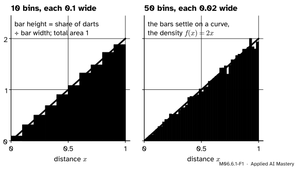
The picture below shows where that curve comes from. Throw 20,000 darts at a round target of radius 1, each equally likely to land anywhere on it, and record each dart’s distance from the centre. Draw a histogram of the distances, scaled so that the area of each bar is the share of darts in it.
M06.6.1-F1
Histograms of 20,000 dart distances, scaled so that bar areas are shares of the darts. With narrower bins the staircase hugs a straight line, the density\({f(x) = 2x}\).
Narrow the bins and the staircase becomes finer, but it does not wander: it settles on one curve. That curve is the probability density function, or density, of the distance. The chance of landing in any interval is the area under the curve over that interval, just as the share of darts in a bar is that bar’s area.
Build it up
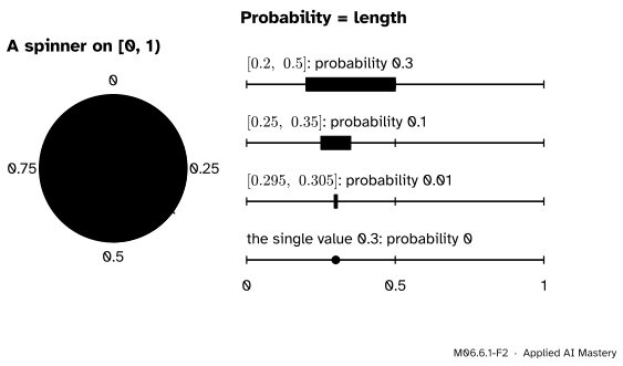
Step 1. Every single value has probability 0. Take the spinner, a pointer on a dial marked from 0 to 1 that stops at a uniformly random point. “Uniform” means that two arcs of the same length are equally likely. Split the dial into 10 equal arcs: each has probability \({1/10}\). Into 1,000: each has \({1/1000}\). The arc around 0.3 can be made as short as you like, so the chance of stopping exactly at 0.3 is smaller than every positive number. It is 0.
M06.6.1-F2
For the spinner an interval’s probability is its length. Shrink the interval around 0.3 and the probability shrinks with it, down to 0 for the single value.
Step 2. Intervals keep their probabilities. The chance of stopping between 0.2 and 0.5 is the share of the dial that arc covers, \({0.5 - 0.2 = 0.3}\). In general, for the spinner and any \({0 \le c \le d \le 1}\),
\[
\Prob(c \le X \le d) = d - c .
\]
There is no contradiction with Step 1. The axioms of M06.1.3 add probabilities over a list of disjoint events, even an infinite list. The points of an interval cannot be put in a list, so adding up their zeros proves nothing about the interval.
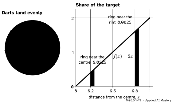
Step 3. Not every variable is spread evenly. Darts land evenly over the target, but not evenly over distances. A thin ring near the rim is longer than a ring of the same width near the centre, so it catches more darts.
M06.6.1-F3
The two rings have the same width, but the outer one covers almost four times as much of the target. On the right, each ring is a strip under the density \({2x}\), and its area is its share.
The target has area \({\pi \cdot 1^2 = \pi}\). The darts that land within distance \(r\) of the centre fill a disc of area \({\pi r^2}\), so \({\Prob(X \le r)} = {\pi r^2 / \pi} = {r^2}\). A ring from \(r\) to \({r + h}\) then holds
The ring from 0.2 to 0.25 holds \({0.0625 - 0.04 = 0.0225}\) of the darts, and the ring from 0.8 to 0.85 holds \({0.7225 - 0.64 = 0.0825}\).
Step 4. Divide by the width. Dividing a ring’s probability by its width \(h\) gives the probability per unit of distance:
\[
\frac{\Prob(r \le X \le r + h)}{h} = 2r + h .
\]
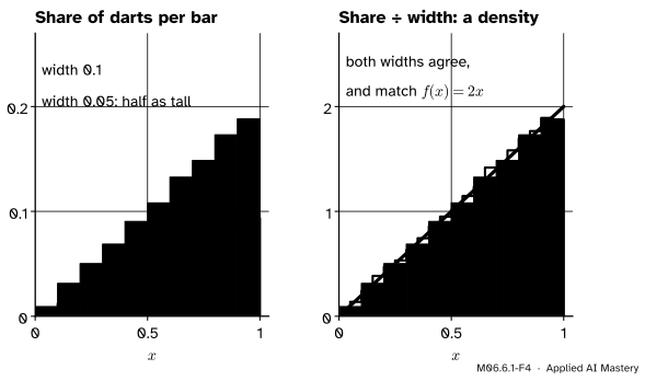
As the ring gets thinner, \({h \to 0}\), this settles on \({2r}\). That limit is the density at \(r\). A histogram does the same division. If each bar’s height were the share of darts in it, halving the bin width would roughly halve every bar. Divide each share by the bin width, and the heights stay put as the bins narrow.
M06.6.1-F4
Left: shares per bar depend on the bin width. Right: shares divided by the width do not, and both histograms sit on the density \({2x}\).
The formal statement
NoteDefinition: density of a continuous random variable
A random variable \(X\) is continuous with density\({f_X}\) if, for all numbers \({a \le b}\),
\[
\Prob(a \le X \le b) = \int_a^b f_X(x)\,dx .
\]
A function \(f\) can be a density exactly when
\({f(x) \ge 0}\) for every \(x\), and
\({\int_{-\infty}^{\infty} f(x)\,dx} = {1}\).
The subscript in \({f_X}\) names the variable; we drop it when only one variable is around. The integral is the area under the graph from \(a\) to \(b\) (M04.5). A density is 0 outside the values \(X\) can take, so the integral over the whole line is really over that range.
Both conditions come from the axioms. If \(f\) were negative on some interval, that interval would get a negative probability. And \({\Prob(-\infty < X < \infty)} = {1}\) because \(X\) is certain to take some value.
Three consequences follow, each in a line.
Single values have probability 0. Put \({a = b}\): \({\Prob(X = a)} = {\int_a^a f(x)\,dx} = {0}\).
End points do not matter. An interval with or without its ends differs by single values, so
\[
\Prob(a < X < b) = \Prob(a \le X \le b).
\]
For a discrete variable this was false, and module M06.5 had to take care over \({<}\) and \({\le}\).
A density is probability per unit of \(x\). For a thin interval of width \(h\) around \(x\), the area under \(f\) is close to a rectangle:
\[
\Prob(x \le X \le x + h) \approx f(x)\,h .
\]
So \({f(x)}\) is a probability divided by a length. It is not the probability of the value \(x\), and nothing stops it from being larger than 1.
M06.6.1-F6
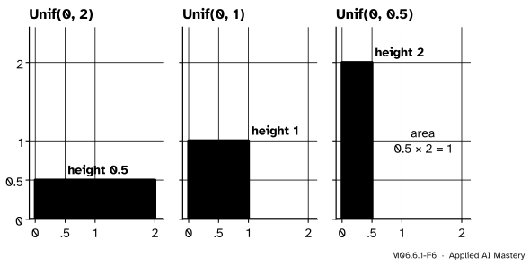
Three uniform densities. Squeezing the same total area of 1 onto a shorter interval makes the density taller: on \({[0, 0.5]}\) its height is 2.
A spinner marked only from 0 to 0.5 has density 2 on that interval, written \({\text{Unif}(0, 0.5)}\). The probabilities are still at most 1: the whole interval has area \({0.5 \times 2 = 1}\).
Worked example
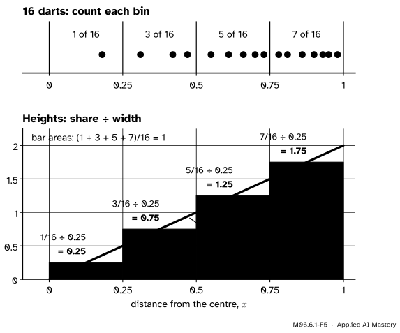
Sixteen darts. A small sample of 16 dart distances, chosen so that the counts come out tidily:
Check the total area. Each bar’s area is its height times 0.25, which gives back its share, so the areas add to \({(1 + 3 + 5 + 7)/16 = 1}\).
M06.6.1-F5
The worked example. Counts become shares, shares divided by the width become heights, and every bar’s top crosses the line \({2x}\) at its middle.
Compare with the density. At the bin midpoints 0.125, 0.375, 0.625 and 0.875 the density \({2x}\) is 0.25, 0.75, 1.25 and 1.75: the bar heights exactly. And the exact chance of the last bin is \({\Prob(0.75 \le X \le 1)} = {1^2 - 0.75^2} = {0.4375} = {\tfrac{7}{16}}\), the share in the sample. A real sample of 16 wobbles around these numbers; this one was picked to hit them, so that every step can be checked by hand.
Code
First the spinner, from scratch: many uniform numbers, and the share that falls in shrinking intervals around 0.3.
import numpy as nprng = np.random.default_rng(0)spins = rng.uniform(0, 1, size=100_000)in_arc = np.mean((spins >=0.2) & (spins <=0.5))print(f"share in [0.2, 0.5]: {in_arc:.4f} (exact 0.3)")for half in (0.05, 0.005, 0.0005): share = np.mean(np.abs(spins -0.3) <= half)print(f"within {half} of 0.3: {share:.5f} (exact {2* half})")print("spins exactly equal to 0.3:", np.sum(spins ==0.3))
share in [0.2, 0.5]: 0.2997   (exact 0.3)
within 0.05 of 0.3: 0.09763   (exact 0.1)
within 0.005 of 0.3: 0.00942   (exact 0.01)
within 0.0005 of 0.3: 0.00099   (exact 0.001)
spins exactly equal to 0.3: 0
The shares shrink with the interval, and not one of 100,000 spins hit 0.3 on the nose. Now the darts: points spread evenly over the square \({[-1, 1]^2}\), kept when they land on the target, and a density-scaled histogram built by hand.
def dart_distances(n, rng):"""Distances from the centre of n darts spread evenly over a target of radius 1.""" kept = []whilelen(kept) < n: x, y = rng.uniform(-1, 1, size=2)if x * x + y * y <=1: kept.append((x * x + y * y) **0.5)return np.array(kept)r = dart_distances(20_000, rng)width =0.1counts = np.zeros(10)for value in r: counts[min(int(value / width), 9)] +=1# which bin of width 0.1heights = counts /len(r) / width # share, divided by widthmids = np.arange(10) * width + width /2print("heights:", np.round(heights, 2))print("2x at the midpoints:", np.round(2* mids, 2))print("total area:", round(float(np.sum(heights * width)), 6))
heights: [0.11 0.31 0.5  0.68 0.9  1.12 1.28 1.49 1.71 1.9 ]
2x at the midpoints: [0.1 0.3 0.5 0.7 0.9 1.1 1.3 1.5 1.7 1.9]
total area: 1.0
The hand-made heights match \({2x}\) at the midpoints to within the sampling wobble, and their total area is 1. NumPy does the same scaling when asked with density=True.
The heights of \({\text{Unif}(0, 0.5)}\) are all close to 2, above 1, while the area is exactly 1.
Explore
This module’s interactive, area under a density, lives in lesson M06.6.3. Try its uniform and \({2x}\) densities now: squeeze the two handles together and watch the probability fall to 0 while the height of the curve stays where it is.
Pitfalls
M06.6.1-F7
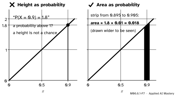
Wrong beside right. The height \({f(0.9) = 1.8}\) is not a probability. The area of a thin strip around 0.9 is: about \({1.8 \times 0.01 = 0.018}\).
“The density at 0.9 is 1.8, so the chance of 0.9 is 1.8.”
The chance of the single value 0.9 is 0. The height 1.8 says that near 0.9 probability is packed at 1.8 per unit of distance, so a strip of width 0.01 there holds about 0.018. Here that is exact: \({0.905^2 - 0.895^2 = 0.018}\). The same slip appears in machine learning: the likelihood of a continuous measurement under a model is a density, so it can be above 1 and its logarithm can be positive. That is not a bug.
“I drew a histogram of counts and the density curve does not fit it.”
Counts grow with the number of samples, and shares shrink with the bin width. Only a histogram scaled to area 1, share divided by width, can be laid over a density. In NumPy that is np.histogram(..., density=True); its heights do not add to 1, their areas do.
“Probability 0 means it cannot happen.”
Every spin lands on some value, and that value had probability 0. For a continuous variable, “probability 0” means “too thin to have area”, not “impossible”.
Check yourself
Recall
1. For a spinner that stops uniformly on \({[0, 1)}\), what is \({\Prob(0.2 \le X \le 0.5)}\), and what is \({\Prob(X = 0.3)}\)?
Show answer
0.3, the length of the interval, and 0.
2. What two conditions must a function meet to be a density?
Show answer
It is never negative, and the total area under it is 1.
3. How do you turn the count in a histogram bar into a density height?
Show answer
Divide the count by the number of samples to get a share, then divide the share by the bin width.
4. Can a density be larger than 1? Give an example.
Show answer
Yes. \({\text{Unif}(0, 0.5)}\) has height 2 on \({[0, 0.5]}\), and its total area is still 1.
5. Why is \({\Prob(a < X < b)}\) the same as \({\Prob(a \le X \le b)}\) for a continuous variable?
Show answer
The two events differ only by the end values \(a\) and \(b\), and each single value has probability 0.
Exercises
1.★ A spinner stops uniformly on \({[0, 1)}\). Find the chance that it stops in \({[0.1, 0.35]}\) or in \({[0.6, 0.7]}\).
Show solution
The two intervals do not overlap, so their probabilities add (M06.1.3): \({(0.35 - 0.1) + (0.7 - 0.6)} = {0.25 + 0.1} = {0.35}\).
2.★★ A histogram of 200 values uses bins of width 0.5. One bin holds 30 values. What is the bar’s height on a density scale? If the bins were made 0.25 wide and the same bin split into two bins of 14 and 16 values, what would their heights be?
Show solution
The share is \({30/200 = 0.15}\), so the height is \({0.15/0.5 = 0.3}\). With width 0.25 the shares are \({14/200 = 0.07}\) and \({16/200 = 0.08}\), and the heights \({0.07/0.25 = 0.28}\) and \({0.08/0.25 = 0.32}\). They sit around 0.3: on a density scale the heights do not halve when the bins do.
3.★★★ For the dart distance, \({\Prob(X \le r) = r^2}\) on \({[0, 1]}\). Use \({\Prob(r \le X \le r + h)/h}\) to find the probability per unit of distance at \({r = 0.5}\) for \({h = 0.1}\) and \({h = 0.01}\), and say what it tends to. Then explain, from the picture of the target, why the density is 0 at the centre.
Show solution
The ratio is \({((r + h)^2 - r^2)/h = 2r + h}\). At \({r = 0.5}\) it is \({1.1}\) for \({h = 0.1}\) and \({1.01}\) for \({h = 0.01}\), tending to \({2r = 1}\), the density \({f(0.5)}\). Near the centre a ring of width \(h\) is a tiny disc of area about \({\pi h^2}\), so its share is about \({h^2}\); divided by \(h\) that is \(h\), which tends to 0. There is very little target close to the centre, so very few darts land there.
Summary card
A density is the curve that area-scaled histograms settle on.
M06.6.1-F1
Narrow the bins and the bars settle on \({f(x) = 2x}\).
Probability is area.\({\Prob(a \le X \le b)} = {\int_a^b f(x)\,dx}\).
A density has \({f \ge 0}\) and total area 1.
Single values have probability 0, so end points never matter.
Height is probability per unit of \(x\): \({\Prob(x \le X \le x + h)} \approx {f(x)\,h}\), and \({f}\) can exceed 1.
In NumPy, np.histogram(..., density=True) divides each share by its bin width.
Sources and next steps
Sources. Each was opened and checked against this lesson on 14 November 2026.
Hossein Pishro-Nik, Introduction to Probability, Statistics, and Random Processes, Section 4.1.0, states that for a continuous random variable \({\Prob(X = x) = 0}\) for every \(x\), and derives the CDF of a value chosen uniformly from \({[a, b]}\). Section 4.1.1 defines the density as the limit of \({\Prob(x < X \le x + \Delta)/\Delta}\), lists its properties (never negative, total area 1, probabilities as integrals) and notes that it can be larger than 1.
Charles M. Grinstead and J. Laurie Snell, Introduction to Probability, second edition, Section 2.2. Example 2.7 is the spinner on \({[0, 1)}\), where single outcomes get probability 0 and \({\Prob(c \le X < d) = d - c}\); Examples 2.9 and 2.12 are the dart’s distance from the centre, with \({\Prob([0, a]) = a^2}\) and density \({2r}\); Definition 2.1 defines a density.
Jeremy Orloff and Jonathan Bloom, Reading 5b, Continuous random variables, MIT OpenCourseWare 18.05, Spring 2022. Section 4 gives the definition and the two properties and says that a density is not a probability and need not be at most 1; Section 4.2 explains its units as probability per unit of \(x\), by analogy with mass and density.
NumPy reference, numpy.histogram: with density=True the result is the value of the density at each bin, normalised so that the integral over the range is 1, and the heights add to 1 only for bins of width 1.
Next.M06.6.2 Probabilities by integration turns “area under the density” into numbers: by hand for the uniform, the dart distance and a waiting time, then with a Riemann sum and scipy.integrate.quad.