Stack the bars of a PMF and you get the CDF, a staircase from 0 to 1 that jumps at each value. Read interval probabilities, medians and quantiles off it, and use it to draw samples from any PMF, the way a language model picks its next word.
M06.5.3L1 Core25 minIn review (what this means)
The maths and code on this page are checked by automated tests on every change, but an independent reader has not signed it off yet. Spot a mistake or a confusing step? Tell us.
Build the CDF of a discrete random variable from its PMF and draw it as a staircase with jumps of size p(x).
Find P(a < X <= b) as F(b) - F(a), and adjust correctly when the inequalities are strict or not.
Read the median and other quantiles off a CDF.
Sample from any PMF by dropping a uniform random number onto the staircase, from scratch and with rng.choice.
The question
A language model has worked out how likely each possible next word is: “mat” 0.5, “floor” 0.25, “sofa” 0.15, “roof” 0.10. Now it must actually pick one, at random but with exactly those chances. A computer’s random number generator only offers uniform numbers between 0 and 1. How do you turn one of those into a word with the right chances?
From the last lesson
1. What two properties does every PMF have?
Show answer
Every bar lies between 0 and 1, and the bars add up to 1.
2. What is the PMF of the bin of a fair Galton board with 4 rows?
Show answer
\({p_X(k) = \binom{4}{k}/16}\): 1, 4, 6, 4 and 1 sixteenths for bins 0 to 4.
Intuition
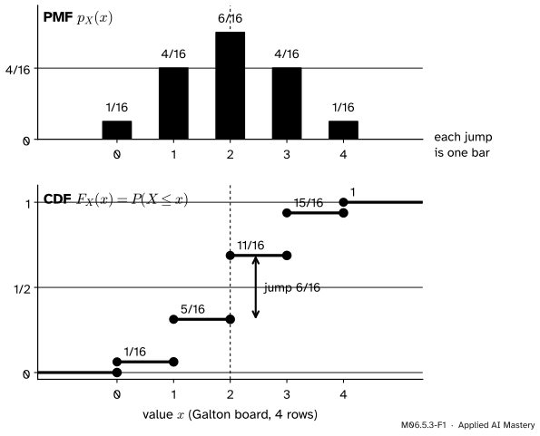
The PMF answers “how likely is exactly \(x\)?”. Often the question is “how likely is at most\(x\)?”: at most 2 errors, a score of 7 or less. Add up the bars from the left as you walk along the number line, and you get a running total that climbs from 0 to 1. That running total is the cumulative distribution function (CDF).
M06.5.3-F1
The CDF stacks the bars. It is flat between the values and jumps at each value by the height of that value’s bar: at 2 it jumps by \(6/16\), the yellow bar.
The staircase holds the same information as the bars: each jump is a bar, so you can read the PMF back off it. What the staircase adds is that sums of neighbouring bars become single readings. “At most 2” is one height, \(11/16\), instead of three bars to add.
Build it up
Step 1. Heights at the values. For the 4-row Galton board, add the bars from the left:
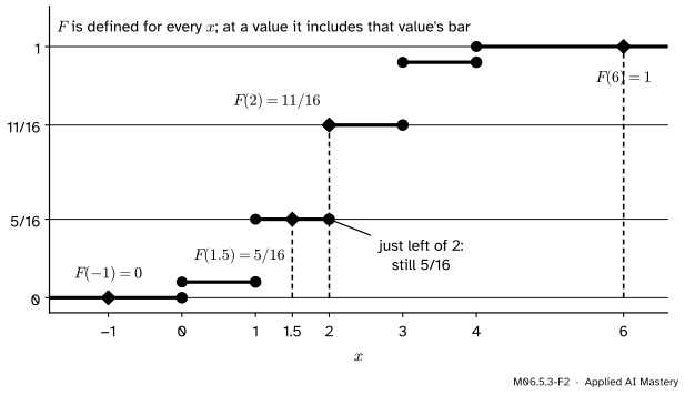
Step 2. Heights between the values.\(F(x)\) is defined for every real \(x\), not just the values \(X\) takes. \({F(1.5) = \Prob(X \leq 1.5)}\), and the values at most 1.5 are 0 and 1, so \({F(1.5) = 5/16}\), the same as \(F(1)\). Below the smallest value the staircase is at 0, since \(X\) is never that small; past the largest it is at 1.
M06.5.3-F2
Reading \(F\) anywhere. Between values it stays flat; at a value it takes the upper level, because “at most 2” includes 2. Just to the left of 2 it is still at \(5/16\).
Step 3. Which end of a jump? At \({x = 2}\), the event “\({X \leq 2}\)” includes \({X = 2}\), so \(F(2)\) is the top of the jump, \(11/16\). That is what the filled dot marks; the hollow dot below it marks the level at points just left of 2. So the CDF of a discrete variable is a staircase that never falls, runs from 0 to 1, and is continuous from the right: at each jump, the value belongs to the upper step.
The formal statement
NoteDefinition: cumulative distribution function
The cumulative distribution function of a random variable \(X\) is
\[
F_X(x) = \Prob(X \leq x)
\]
for every real number \(x\). For a discrete \(X\) it is the sum of the bars at or to the left of \(x\): \({F_X(x)} = {\sum_{t \leq x} p_X(t)}\), the sum taken over values \(t\) of \(X\).
It never falls. If \({a < b}\), every outcome with \({X \leq a}\) also has \({X \leq b}\), so \({\{X \leq a\}}\) lies inside \({\{X \leq b\}}\). By lesson M06.1.4 a smaller event cannot have a larger probability, so \({F(a) \leq F(b)}\).
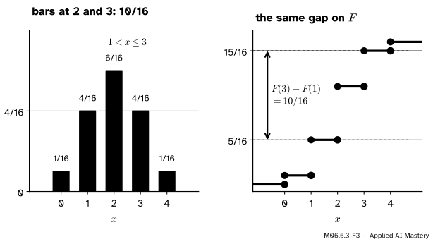
Intervals are differences. Take \({a < b}\). The event \({\{X \leq b\}}\) splits into two disjoint pieces, \({X \leq a}\) and \({a < X \leq b}\). By additivity, \({F(b)} = {F(a) + \Prob(a < X \leq b)}\), so
\[
\Prob(a < X \leq b) = F(b) - F(a).
\]
M06.5.3-F3
The same probability twice: the yellow bars over \({1 < x \leq 3}\) on the left, the gap between two levels of the staircase on the right.
Jumps are bars. The size of the jump at a value \(x\) is \(p_X(x)\), so for a variable whose values are whole numbers, \({p_X(x) = F(x) - F(x - 1)}\). The CDF determines the PMF, and the PMF the CDF.
Strict or not. Because a single value can carry probability, \({<}\) and \({\leq}\) differ. Adding or removing one bar fixes each case:
\[
\begin{aligned}
\Prob(X < b) &= F(b) - p_X(b), \\
\Prob(a \leq X \leq b) &= F(b) - F(a) \\
&\quad + p_X(a).
\end{aligned}
\]
For the 4-row board: \({\Prob(X < 2)} = {11/16 - 6/16} = {5/16}\), which is \(F(1)\), as it should be.
Quantiles. For a number \(q\) between 0 and 1, the \(q\)-quantile is the smallest value \(x\) with \({F(x) \geq q}\): go across from height \(q\) until you meet the staircase, then down. The median is the \(1/2\)-quantile. On the 4-row board, \({F(1) = 5/16}\) is below \(1/2\) and \({F(2) = 11/16}\) is not, so the median is 2.
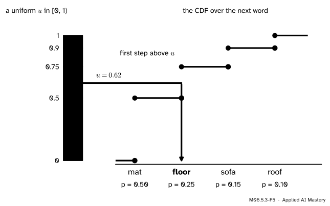
Sampling. Here is the answer to the question. List the values \({x_1 < x_2 < \dots}\), draw \(U\) uniform on \({[0, 1)}\), and return the first \(x_k\) whose height \(F(x_k)\) is greater than \(U\). The value \(x_k\) comes out exactly when \(U\) lands in the slice from \({F(x_{k-1})}\) up to (but not including) \(F(x_k)\). A uniform number lands in a slice with probability equal to its length, so
Sampling a word. The uniform number 0.62 lies in the slice that belongs to “floor”, the first word whose step is above 0.62. Each word owns a slice as long as its chance.
Go deeper: when two numbers could both claim to be the median
If \(F\) sits exactly at \(1/2\) on a flat stretch, any number on that stretch splits the probability in half. For one fair coin flip, \({X \in \{0, 1\}}\), \({F(0) = 1/2}\), and every number strictly between 0 and 1 has exactly half the probability below it and half above it. The rule “smallest \(x\) with \({F(x) \geq q}\)” picks 0; other books take the midpoint, 0.5. Software varies too, so check which rule a library uses.
Worked example
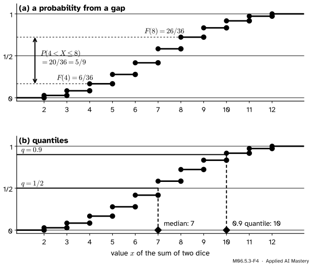
The sum of two dice. Find \({\Prob(4 < X \leq 8)}\), \({\Prob(4 \leq X \leq 8)}\), the median and the 0.9-quantile.
The CDF. Add the counts \({1, 2, 3, 4, 5, 6, 5, 4, 3, 2, 1}\) from the left. In 36ths, \(F\) at \({x = 2, 3, \dots, 12}\) is
Median.\({F(6) = 15/36}\) is below \(1/2\) and \({F(7) = 21/36}\) is not, so the median is 7.
0.9-quantile.\({F(9) = 30/36 \approx 0.833}\) is below 0.9 and \({F(10)} = {33/36 \approx 0.917}\) is not, so the 0.9-quantile is 10. At least 90% of rolls give 10 or less.
Code
From scratch: the CDF is a running total, numpy.cumsum. Read a gap and two quantiles off it.
import numpy as npfrom fractions import Fractionfrom itertools import accumulatevalues =list(range(2, 13))counts = [6-abs(x -7) for x in values]F = {x: Fraction(c, 36) for x, c inzip(values, accumulate(counts))} # exact running totalsdef quantile(q):"""Smallest value x with F(x) >= q."""returnnext(x for x in values if F[x] >= q)print("F:", [str(F[x]) for x in values])print("P(4 < X <= 8) =", F[8] - F[4], " P(4 <= X <= 8) =", F[8] - F[3])print("median:", quantile(Fraction(1, 2)), " 0.9-quantile:", quantile(Fraction(9, 10)))print("cumsum in floats:", np.cumsum(counts) /36)
Now the sampler. numpy.searchsorted(cdf, u, side="right") returns the index of the first entry of cdf that is greater than u, which is exactly the rule. Rounding can leave the last running total a hair below 1, so set it to 1 by hand; otherwise a u very close to 1 could fall off the end.
words = np.array(["mat", "floor", "sofa", "roof"])probs = np.array([0.5, 0.25, 0.15, 0.10])cdf = np.cumsum(probs)cdf[-1] =1.0# guard against roundingdef sample(u):return words[np.searchsorted(cdf, u, side="right")]for u in (0.31, 0.62, 0.80, 0.93):print(u, "->", sample(u))rng = np.random.default_rng(11)draws = sample(rng.random(100_000)) # 100,000 uniform numbers at onceshares = np.array([np.mean(draws == w) for w in words])print("from scratch:", shares.round(3))
0.31 -> mat
0.62 -> floor
0.8 -> sofa
0.93 -> roof
from scratch: [0.501 0.25  0.15  0.1  ]
The library does the same job in one call: rng.choice with the argument p draws from a PMF.
library = rng.choice(words, size=100_000, p=probs)lib_shares = np.array([np.mean(library == w) for w in words])print("rng.choice: ", lib_shares.round(3))
rng.choice: [0.499 0.25 0.151 0.1 ]
Both sets of shares sit within a hundredth of 0.5, 0.25, 0.15 and 0.10. A language model does this once for every word it writes, with a PMF over tens of thousands of words (course A02 adds the temperature and top-p settings that reshape that PMF first).
Explore
The Galton board lives in lesson M06.5.2. Set 4 rows and drop a few hundred balls, then add the shares of bins 0, 1 and 2: that running total is your simulated \(F(2)\), and it should be close to \(11/16\), about 0.69.
Pitfalls
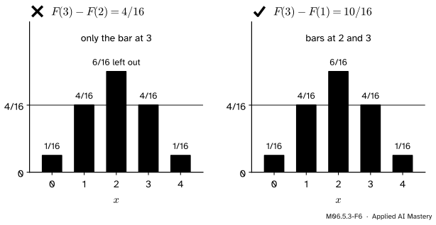
M06.5.3-F6
Wrong beside right, for \({\Prob(2 \leq X \leq 3)}\). Subtracting \(F(2)\) removes the bar at 2 as well; to keep it, subtract \(F(1)\).
“\({\Prob(2 \leq X \leq 3)} = {F(3) - F(2)}\).”
\({F(3) - F(2)}\) is \({\Prob(2 < X \leq 3)}\): the bar at 2 is inside \(F(2)\), so subtracting it takes that bar away. For whole-number values, \({\Prob(a \leq X \leq b)} = {F(b) - F(a - 1)}\). On the board, that is \({15/16 - 5/16 = 10/16}\), not \(4/16\). For a continuous variable the two answers agree (M06.6), which is why the slip is easy to carry over.
“Join the dots: the CDF rises smoothly from one value to the next.”
A discrete \(X\) takes no values between 1 and 2, so \({\Prob(X \leq 1.5)}\) equals \({\Prob(X \leq 1)}\) and the CDF is flat there. Drawing ramps between the dots would say that values like 1.5 carry probability. Only the staircase is right.
“To sample, compare \(U\) with each probability on its own.”
Testing “\({U < 0.5}\)? then mat; \({U < 0.25}\)? then floor …” uses the bars instead of their running totals, and gets the chances wrong: “floor” would never be picked, since any \(U\) below 0.25 is already below 0.5. The slices must be stacked end to end, which is what the cumulative sums do.
Check yourself
Recall
1. Define the CDF of \(X\).
Show answer
\({F_X(x) = \Prob(X \leq x)}\) for every real number \(x\).
2. What does the CDF of a discrete variable look like?
Show answer
A staircase that starts at 0, never falls, ends at 1, is flat between the values, and jumps at each value \(x\) by \(p_X(x)\), taking the upper level at the jump.
3. Write \({\Prob(a < X \leq b)}\) in terms of \(F\).
Show answer
\({F(b) - F(a)}\).
4. How do you read the median off a CDF?
Show answer
Go across from height \(1/2\) until you meet the staircase, then down: the median is the smallest value \(x\) with \({F(x) \geq 1/2}\).
5. How does the inverse-CDF sampler turn a uniform \(U\) into a value of \(X\)?
Show answer
It returns the first value \(x_k\) whose height \(F(x_k)\) is greater than \(U\). Each value owns a slice of \({[0, 1)}\) as long as its probability, so it is returned with that probability.
Exercises
1.★ For the 4-row Galton board, find \({\Prob(X \geq 2)}\) and \({\Prob(1 \leq X \leq 3)}\) from the CDF.
Show solution
\({\Prob(X \geq 2)}\) is the complement of \({X \leq 1}\), so it is \({1 - F(1)} = {1 - 5/16} = {11/16}\). For \({1 \leq X \leq 3}\) the bar at 1 is included, so subtract the level below it: \({F(3) - F(0)} = {15/16 - 1/16} = {14/16} = {7/8}\).
2.★★ Let \(M\) be the larger of two dice. Use the corner square of lesson M06.5.1 to find \(F_M(m)\) for \({m = 1, \dots, 6}\), get the PMF from the jumps, and find the median of \(M\).
Show solution
\({M \leq m}\) exactly when both dice are at most \(m\): an \(m\) by \(m\) square of \({m^2}\) cells, so \({F_M(m) = m^2/36}\). The jumps are
which matches exercise 1 of lesson M06.5.2. For the median, \({F(4) = 16/36}\) is below \(1/2\) and \({F(5) = 25/36}\) is not, so the median is 5.
3.★★★ A PMF puts 0.2 on the value 0, 0.5 on 1 and 0.3 on 2. Build the cumulative sums, and say which value the sampler returns for \({u = 0.05}\), \({u = 0.55}\), \({u = 0.7}\) and \({u = 0.97}\). Then list the values in the order 2, 1, 0 instead, and sample the same four numbers. Do the samples change? Does the distribution of the samples change?
Show solution
In the order 0, 1, 2 the running totals are 0.2, 0.7 and 1. The rule returns the first value whose total is greater than \(u\): \({u = 0.05}\) gives 0, \({u = 0.55}\) gives 1, \({u = 0.7}\) gives 2 (the total at 1 is 0.7, which is not greater than 0.7), and \({u = 0.97}\) gives 2.
In the order 2, 1, 0 the running totals are 0.3, 0.8 and 1, so the same numbers give 2, 1, 1 and 0. The individual samples change, because the slices sit in a different order. The distribution does not: each value still owns a slice of length equal to its probability (2 owns \({[0, 0.3)}\), 1 owns \({[0.3, 0.8)}\), 0 owns \({[0.8, 1)}\)), so each is returned with the same chance as before.
Summary card
The CDF is the staircase of running totals of the PMF.
M06.5.3-F1
Each jump is one bar.
Definition.\({F_X(x) = \Prob(X \leq x)}\), for every real \(x\).
Shape. Never falls, from 0 to 1, jumps by \(p_X(x)\) at each value.
Intervals.\({\Prob(a < X \leq b)} = {F(b) - F(a)}\); mind \({<}\) and \({\leq}\).
Quantile. The smallest \(x\) with \({F(x) \geq q}\); the median is \({q = 1/2}\).
Sampling. Return the first value whose \(F\) exceeds a uniform \(U\).
Sources and next steps
Sources. Each was opened and checked against this lesson on 14 November 2026.
Hossein Pishro-Nik, Introduction to Probability, Statistics, and Random Processes, Section 3.2.1. The definition \({F_X(x) = P(X \leq x)}\) for all real \(x\); equation (3.1), \({P(a < X \leq b)} = {F_X(b) - F_X(a)}\); the CDF of a discrete variable as a staircase that jumps by \(P_X(x_k)\) at each value; and that a CDF never decreases and approaches 1.
Jeremy Orloff and Jonathan Bloom, Reading 4a: Discrete Random Variables, MIT OpenCourseWare 18.05, Spring 2022. Section 2.6 defines the cdf with “less than or equal to” and warns that this matters for exact answers; its table for the maximum of two dice reads 1/36, 4/36, 9/36, 16/36, 25/36, 36/36, the squares of exercise 2.
NumPy documentation, numpy.searchsorted (with side="right" the returned index \(i\) satisfies a[i-1] <= v < a[i]) and numpy.random.Generator.choice (the argument p gives the probabilities of the entries, which must sum to 1).