\( \newcommand{\vect}[1]{\boldsymbol{\mathbf{#1}}} \newcommand{\mat}[1]{\boldsymbol{\mathbf{#1}}} \newcommand{\R}{\mathbb{R}} \newcommand{\E}{\mathbb{E}} \newcommand{\Prob}{\mathbb{P}} \newcommand{\T}{^{\top}} \newcommand{\norm}[1]{\lVert #1 \rVert} \newcommand{\abs}[1]{\lvert #1 \rvert} \newcommand{\ihat}{\mkern1mu\hat{\boldsymbol{\imath}}\mkern2mu} \newcommand{\jhat}{\mkern1mu\hat{\boldsymbol{\jmath}}\mkern2mu} \newcommand{\pd}[2]{\frac{\partial #1}{\partial #2}} \newcommand{\argmax}{\operatorname*{arg\,max}} \newcommand{\argmin}{\operatorname*{arg\,min}} \newcommand{\cdata}[1]{\class{c-data}{#1}} \newcommand{\cmodel}[1]{\class{c-model}{#1}} \newcommand{\ctruth}[1]{\class{c-truth}{#1}} \newcommand{\cgrad}[1]{\class{c-grad}{#1}} \newcommand{\closs}[1]{\class{c-loss}{#1}} \newcommand{\cparam}[1]{\class{c-param}{#1}} \newcommand{\csecond}[1]{\class{c-second}{#1}} \renewcommand{\,}{\mkern3mu} \)

Independence

Two events are independent when learning one leaves the chance of the other where it was. Define independence by a product, prove it matches the conditional picture, tell pairwise from mutual independence, and meet conditional independence, the assumption behind every likelihood that is a product.

M06.3.4L1 Core25 min

In review

The maths and code on this page are checked by automated tests on every change, but an independent reader has not signed it off yet. Spot a mistake or a confusing step? Tell us.

Before this lesson: M06.3.3 The law of total probability

What you will be able to do

Define independence of two events by P(A and B) = P(A) P(B), and prove that it is the same as P(A | B) = P(A) when P(B) > 0.
Test a pair of events for independence by computing both sides, on the dice grid and from a table.
Explain why disjoint events with positive probability are never independent.
Distinguish pairwise from mutual independence for three events, with an example where they differ.
Define conditional independence and compute with it on two repeated tests, and explain why independent trials let a likelihood be a product.

The question

A classifier is right on 90% of examples. On a test set of 10 examples, what is the chance that it gets all 10 right? Almost everyone writes \({0.9^{10} \approx 0.349}\) without a second thought. That multiplication is a claim about the examples: that how the model does on one tells you nothing about how it does on another. When is that claim true, how do you check it, and what goes wrong when it fails?

From the last lesson

1. State the law of total probability for the partition \(B\), \(B^c\).

Show answer

\({\Prob(A)} = {\Prob(A \mid B)\,\Prob(B)} + {\Prob(A \mid B^c)\,\Prob(B^c)}\).

2. Why must \({\Prob(A)}\) lie between \({\Prob(A \mid B)}\) and \({\Prob(A \mid B^c)}\)?

Show answer

Because it is their weighted average, with weights \({\Prob(B)}\) and \({\Prob(B^c)}\) that are not negative and add to 1.

Intuition

Lesson M06.3.3 showed that \(\Prob(A)\) is a weighted average of two shares: the share of \(A\) inside \(B\) and the share of \(A\) outside \(B\). Usually the shares differ, and learning whether \(B\) happened moves your belief about \(A\) up or down. Sometimes they are the same. Then learning \(B\) moves nothing, and we call \(A\) and \(B\) independent.

M06.3.4-F1

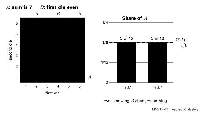
Roll two dice. Event \(A\) is “the sum is 7” and \(B\) is “the first die is even”. Three of the 18 outcomes in \(B\) have sum 7, and so do three of the 18 outside \(B\). The shares are level, so they both equal \({\Prob(A) = 1/6}\).

This may surprise you, since the sum certainly depends on the first die. But “the sum is 7” asks only whether the second die is the one face that completes 7, and for every first die there is exactly one such face. Whatever the first die shows, the chance is \(1/6\). Independence is a fact about the numbers, not about whether one die “affects” the event.

Build it up

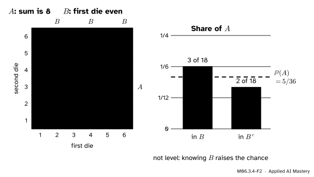
Step 1. Change the event. Keep \(B\) and make \(A\) “the sum is 8”. Now the first die matters: if it is 1, no second die gives 8.

Step 2. Compare the shares. Inside \(B\) the outcomes with sum 8 are (2, 6), (4, 4) and (6, 2): 3 of 18. Outside \(B\) they are (3, 5) and (5, 3): 2 of 18.

Step 3. Read the verdict. The shares are not level. Learning that the first die is even raises the chance of 8 from \({\Prob(A) = 5/36}\) to \({3/18 = 6/36}\). These events are dependent.

M06.3.4-F2

The same \(B\) with a different \(A\). The two shares differ, and \(\Prob(A)\) sits between them, as the law of total probability says it must.

So independence is not a property of an event on its own. It is a property of a pair: “sum is 7” is independent of “first die even”, but “sum is 8” is not.

The formal statement

“Learning \(B\) does not change the chance of \(A\)” is \({\Prob(A \mid B) = \Prob(A)}\). Multiply both sides by \({\Prob(B)}\) and the left side becomes \({\Prob(A \cap B)}\), by the multiplication rule. That product form is the one we take as the definition, because it is symmetric in \(A\) and \(B\) and needs no division.

Definition: independent events

Events \(A\) and \(B\) are independent if

\[ \Prob(A \cap B) = \Prob(A)\,\Prob(B) . \]

Otherwise they are dependent.

Theorem. If \({\Prob(B) > 0}\), then \(A\) and \(B\) are independent exactly when \({\Prob(A \mid B) = \Prob(A)}\).

Proof. Suppose they are independent. Then \({\Prob(A \mid B)} = {\Prob(A \cap B)/\Prob(B)} = {\Prob(A)\,\Prob(B)/\Prob(B)} = {\Prob(A)}\). Conversely, suppose \({\Prob(A \mid B) = \Prob(A)}\). Then the multiplication rule gives \({\Prob(A \cap B)} = {\Prob(B)\,\Prob(A \mid B)} = {\Prob(B)\,\Prob(A)}\). \(\square\)

By the same argument with the roles swapped, \({\Prob(B \mid A) = \Prob(B)}\) when \({\Prob(A) > 0}\). In the area picture, independence says that \(A\) takes the same share of the strip \(B\) as of the whole square: the two cuts in the zoom-in square are level.

Complements come for free. If \(A\) and \(B\) are independent, so are \(A\) and \(B^c\). The set \(A\) splits into the disjoint pieces \({A \cap B}\) and \({A \cap B^c}\), so

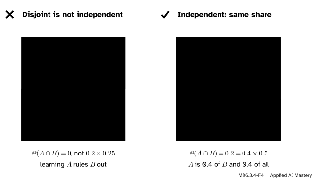
\[ \begin{aligned} \Prob(A \cap B^c) &= \Prob(A) - \Prob(A \cap B) \\ &= \Prob(A) - \Prob(A)\,\Prob(B) \\ &= \Prob(A)\,\big(1 - \Prob(B)\big) \\ &= \Prob(A)\,\Prob(B^c). \end{aligned} \]

Disjoint is the opposite of independent. If \(A\) and \(B\) are disjoint and both have positive probability, then \({\Prob(A \cap B) = 0}\) while \({\Prob(A)\,\Prob(B) > 0}\). They are dependent, and strongly so: learning \(A\) tells you for certain that \(B\) did not happen.

Three or more events. For three events, independence of each pair is not enough.

Definition: mutual independence

Events \(A\), \(B\), \(C\) are mutually independent if all four of these hold:

\[ \begin{aligned} \Prob(A \cap B) &= \Prob(A)\,\Prob(B), \\ \Prob(A \cap C) &= \Prob(A)\,\Prob(C), \\ \Prob(B \cap C) &= \Prob(B)\,\Prob(C), \\ \Prob(A \cap B \cap C) &= \Prob(A)\,\Prob(B)\,\Prob(C). \end{aligned} \]

For \(n\) events, the product rule must hold for every collection of two or more of them.

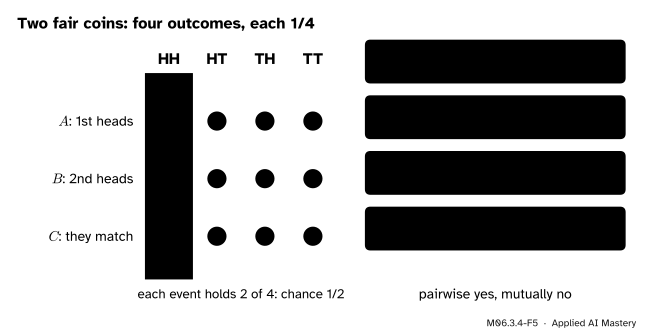
If only the first three hold, the events are pairwise independent. Two fair coins show the gap.

M06.3.4-F5

Each pair of events shares exactly one outcome, HH, so each pair is independent. All three share the same outcome, so the triple product fails: knowing \(A\) and \(B\) makes \(C\) certain.

Conditional independence. Events can be independent inside each part of a partition without being independent overall.

Definition: conditional independence

\(A\) and \(B\) are conditionally independent given \(C\), where \({\Prob(C) > 0}\), if

\[ \Prob(A \cap B \mid C) = \Prob(A \mid C)\,\Prob(B \mid C). \]

This is plain independence for the probability \({\Prob(\,\cdot \mid C)}\) of M06.3.1. Take the test of M06.3.3 and test each person twice. Suppose the two results are independent given the person’s state: given the condition, each is positive with chance 0.9; given no condition, with chance 0.1. The law of total probability, with conditional independence inside each branch, gives

\[ \begin{aligned} &\Prob(\text{both pos}) \\ &\quad= 0.9^2 \times 0.01 + 0.1^2 \times 0.99 \\ &\quad= 0.0081 + 0.0099 = 0.018 . \end{aligned} \]

But \({\Prob(\text{pos})^2} = {0.108^2} = {0.011664}\). The two results are not independent overall: \({\Prob(\text{2nd pos} \mid \text{1st pos})} = {0.018/0.108} = {1/6}\), well above 0.108. A first positive makes the condition more likely, and that makes a second positive more likely. Lesson M06.4.3 uses exactly this assumption to update twice.

Independent trials multiply. When trials are mutually independent, the chance of any sequence of results is the product of the chances of each. That is why ten examples, each right with chance 0.9 and independent of one another, are all right with chance \({0.9^{10} \approx 0.349}\), and why the likelihood of a data set under a model is a product over the examples (ML01.6.2). Naive Bayes (ML02.6) goes one step further and assumes the words of an email are conditionally independent given its label.

Worked example

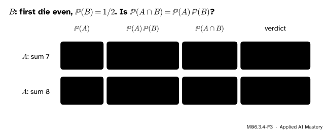
Test two pairs of dice events for independence. Let \(B\) be “the first die is even”, so \({\Prob(B) = 18/36 = 1/2}\). Test it against \(A_7\), “the sum is 7”, and \(A_8\), “the sum is 8”.

Sum 7. Six outcomes have sum 7, so \({\Prob(A_7) = 6/36 = 1/6}\). Three of them, (2, 5), (4, 3) and (6, 1), have an even first die, so \({\Prob(A_7 \cap B) = 3/36 = 1/12}\). The product is \({\Prob(A_7)\,\Prob(B)} = {1/6} \times {1/2} = {1/12}\). Equal: independent.

Sum 8. Five outcomes have sum 8, so \({\Prob(A_8) = 5/36}\). Three have an even first die, so \({\Prob(A_8 \cap B) = 3/36 = 6/72}\). The product is \({5/36 \times 1/2 = 5/72}\). Not equal: dependent.

M06.3.4-F3

The product test, one row per pair. Write both sides over the same denominator before comparing.

Cross-check by conditioning. \({\Prob(A_7 \mid B)} = {3/18} = {1/6} = {\Prob(A_7)}\), while \({\Prob(A_8 \mid B)} = {3/18} = {1/6} \ne {5/36}\). The two tests agree, as the theorem promised.

Code

From scratch: a test of the product rule on any finite, equally likely sample space, with exact fractions so that “equal” means equal.

from fractions import Fraction
from itertools import product

omega = set(product(range(1, 7), repeat=2))

def P(event):
    return Fraction(len(event), len(omega))

def independent(a, b):
    return P(a & b) == P(a) * P(b)

first_even = {w for w in omega if w[0] % 2 == 0}
verdicts = {s: independent({w for w in omega if sum(w) == s}, first_even) for s in range(2, 13)}
print("sum 7:", verdicts[7], "  sum 8:", verdicts[8])
print("independent of 'first die even':", [s for s, ok in verdicts.items() if ok])

sum 7: True   sum 8: False
independent of 'first die even': [3, 5, 7, 9, 11]

Every odd sum passes and every even sum fails. An odd sum needs one even die and one odd die, so swapping the two dice turns each outcome of the event with an even first die into one with an odd first die: the two shares are always level. Next, the two coins.

coins = set(product("HT", repeat=2))
Q = lambda e: Fraction(len(e), len(coins))
A = {w for w in coins if w[0] == "H"}
B = {w for w in coins if w[1] == "H"}
C = {w for w in coins if w[0] == w[1]}
pairs_ok = all(Q(x & y) == Q(x) * Q(y) for x, y in [(A, B), (A, C), (B, C)])
triple = Q(A & B & C), Q(A) * Q(B) * Q(C)
print("every pair independent:", pairs_ok, "  triple:", triple[0], "vs", triple[1])

every pair independent: True   triple: 1/4 vs 1/8

Now conditional independence, simulated: each person gets two tests that are independent given their state.

import numpy as np

rng = np.random.default_rng(seed=34)
n = 1_000_000
sick = rng.random(n) < 0.01
p = np.where(sick, 0.9, 0.1)
first, second = rng.random(n) < p, rng.random(n) < p     # independent given the state
both = (first & second).mean()
print("P(both positive):", round(both, 4), "  P(positive)^2:", round(first.mean() ** 2, 4))
print("P(2nd positive | 1st positive):", round(second[first].mean(), 3))

exact_both = 0.9**2 * 0.01 + 0.1**2 * 0.99
all_right = 0.9**10                                     # ten independent examples
print("exact:", round(exact_both, 4), " all 10 right:", round(all_right, 3))

P(both positive): 0.018   P(positive)^2: 0.0117
P(2nd positive | 1st positive): 0.167
exact: 0.018  all 10 right: 0.349

The simulated values match \({0.018}\) and \({1/6}\) to the shown digits, give or take the seed; the products of the plain chances do not.

Explore

This module’s interactive, the zoom-in square, lives in lesson M06.3.3. Press Make the shares level: the two cuts line up, the dashed line for \(\Prob(A)\) runs straight along them, and the read-out says the events are independent and checks \({\Prob(A \cap B) = \Prob(A)\,\Prob(B)}\). Then move one share by a single step and watch the verdict change.

Pitfalls

M06.3.4-F4

Wrong beside right. Disjoint events cannot happen together, which is strong information. Independent events overlap in exactly the proportion that leaves each one’s share unchanged.

“Disjoint events are independent: they have nothing to do with each other.”

They have everything to do with each other: if one happens, the other cannot. For events of positive probability, disjoint means \({\Prob(A \cap B) = 0 < \Prob(A)\,\Prob(B)}\), so they are dependent.

“If every pair is independent, the whole set is.”

Not so: with two fair coins, “first heads”, “second heads” and “they match” are pairwise independent, but any two of them decide the third. Checking the product of all three alone is not enough either (Exercise 3). Mutual independence needs every collection.

“Independent given the state means independent.”

Two test results can be independent given the person’s state and still dependent for a person picked at random, because the state they share links them: 0.018 against \({0.108^2 \approx 0.0117}\). Treating repeated measurements of one patient, or several rows from one user, as independent overstates how much evidence they carry. It is also why a data set with several rows per person is split into training and test sets by person, not by row.

Check yourself

Recall

1. Define independence of two events.

Show answer

\({\Prob(A \cap B) = \Prob(A)\,\Prob(B)}\).

2. When \({\Prob(B) > 0}\), what is independence in terms of conditional probability?

Show answer

\({\Prob(A \mid B) = \Prob(A)}\): learning \(B\) leaves the chance of \(A\) unchanged.

3. On the dice grid, are “sum is 7” and “first die even” independent? And “sum is 8” with “first die even”?

Show answer

Yes: \({3/36 = 1/6 \times 1/2}\). No: \({3/36 = 6/72}\) but \({5/36 \times 1/2 = 5/72}\).

4. Why are disjoint events with positive probabilities never independent?

Show answer

Their intersection has probability 0, but the product of their probabilities is positive.

5. What extra condition turns pairwise independence of \(A\), \(B\), \(C\) into mutual independence?

Show answer

\({\Prob(A \cap B \cap C)} = {\Prob(A)\,\Prob(B)\,\Prob(C)}\).

Exercises

1. ★ A card is drawn from a shuffled deck of 52. Are “it is an ace” and “it is a heart” independent?

Show solution

\({\Prob(\text{ace}) = 4/52 = 1/13}\), \({\Prob(\text{heart}) = 13/52 = 1/4}\) and \({\Prob(\text{ace of hearts})} = {1/52}\). Since \({1/13 \times 1/4 = 1/52}\), they are independent: an ace is as likely among the hearts (1 of 13) as in the whole deck (4 of 52).

2. ★★ Prove that if \(A\) and \(B\) are independent, so are \(A^c\) and \(B^c\). Check it on “sum is 7” and “first die even”.

Show solution

By the result in the formal statement, \(A\) and \(B^c\) are independent. Apply the same result to the pair \(B^c\), \(A\) (independence is symmetric): \(B^c\) and \(A^c\) are independent. On the dice: “sum not 7” and “first die odd” share the 18 outcomes with an odd first die except the three with sum 7, so \({\Prob = 15/36}\); and \({\Prob(\text{not 7})\,\Prob(\text{odd})} = {5/6} \times {1/2} = {15/36}\).

3. ★★★ Let \({\Omega = \{a, b, c, d, e, f\}}\) with \({\Prob(a) = \Prob(b) = 1/8}\) and \({\Prob(c)} = {\Prob(d)} = {\Prob(e)} = {\Prob(f)} = {3/16}\). Let \({A = \{d, e, a\}}\), \({B = \{c, e, a\}}\) and \({C = \{c, d, a\}}\). Show that \({\Prob(A \cap B \cap C)} = {\Prob(A)\,\Prob(B)\,\Prob(C)}\) but that no two of the events are independent.

Show solution

\({\Prob(A)} = {3/16} + {3/16} + {1/8} = {1/2}\), and in the same way \({\Prob(B) = \Prob(C) = 1/2}\). The three share only \(a\), so \({\Prob(A \cap B \cap C)} = {1/8} = {(1/2)^3}\). But \({A \cap B = \{e, a\}}\) has probability \({3/16 + 1/8 = 5/16}\), not \({1/4}\); likewise \({A \cap C = \{d, a\}}\) and \({B \cap C = \{c, a\}}\) each have \({5/16}\). So the triple product holds while every pair is dependent. This example is Exercise 8 of Grinstead and Snell, section 4.1.

Summary card

Independent: learning one event leaves the chance of the other where it was.

The anchor figure again: the dice grid with the sum-7 diagonal and the even first-die columns, beside two level bars, 3 of 18 in B and 3 of 18 outside B, both at P(A) = 1/6. — M06.3.4-F1
Level shares mean independence.

Definition. \({\Prob(A \cap B) = \Prob(A)\,\Prob(B)}\); equally \({\Prob(A \mid B) = \Prob(A)}\) when \({\Prob(B) > 0}\).
Disjoint events of positive probability are dependent.
Mutual independence needs every collection; pairwise is weaker.
Conditional independence given \(C\) does not give independence: 0.018 against 0.0117.
Independent trials multiply: \({0.9^{10} \approx 0.349}\).

Sources and next steps

Sources. Each was opened and checked against this lesson on 14 November 2026.

Charles M. Grinstead and J. Laurie Snell, Introduction to Probability, second edition. Section 4.1: Definition 4.1 and Theorem 4.1 (independent exactly when \({\Prob(E \cap F) = \Prob(E)\,\Prob(F)}\)), Definition 4.2 (mutual independence over every subset), Exercise 7 (two tosses and whether they match: pairwise but not mutually independent) and Exercise 8 (the six-point example of Exercise 3 above).
Hossein Pishro-Nik, Introduction to Probability, Statistics, and Random Processes, Section 1.4.1 (the product definition, \({\Prob(A \mid B) = \Prob(A)}\), disjoint events of positive probability are not independent, and the four equations for three events) and Section 1.4.4 (conditional independence, with an example of events independent given \(C\) but dependent overall).
Jeremy Orloff and Jonathan Bloom, Reading 3: Conditional Probability, Independence and Bayes’ Theorem, MIT OpenCourseWare 18.05, Spring 2022. Section 6 gives equation (6), the product definition, and shows it equals \({\Prob(A \mid B) = \Prob(A)}\) when \({\Prob(B) \ne 0}\).
Marc Peter Deisenroth, A. Aldo Faisal and Cheng Soon Ong, Mathematics for Machine Learning, Section 6.4.5: independence of random variables (Definition 6.10) and conditional independence (Definition 6.11), in the notation the machine-learning courses use.

Next. M06.4 turns conditional probabilities round with Bayes’ rule, and M06.4.3 updates twice on two test results that are independent given the person’s state. M06.5.4 carries independence from events to random variables.

This lesson unlocks

M06.4.3 Odds, likelihood ratios and updating twice M06.5.4 Independent random variables and their sums

Your progress is saved in this browser only. No account, no tracking.