A probability gives every event a number under three rules: never negative, one for the whole sample space, and adding up over events that cannot happen together. See them as areas, use them on a loaded die and on flips until the first head, and meet two readings of the same number.
M06.1.3L1 Core25 minIn review (what this means)
The maths and code on this page are checked by automated tests on every change, but an independent reader has not signed it off yet. Spot a mistake or a confusing step? Tell us.
State the three axioms of probability, and check whether a proposed assignment of probabilities obeys them.
Compute the probability of an event on a finite sample space as the sum of the probabilities of its outcomes, for a fair and for a loaded die.
Use additivity over countably many events, with the geometric sum, to find probabilities for flips until the first head.
Explain the long-run frequency and the degree-of-belief readings of a probability, and simulate a relative frequency settling down.
The question
A weather app says 30% chance of rain. An image classifier says “cat 0.92”. A spam filter says 0.7. Each is a number between 0 and 1, but that alone does not make it a probability. What does? The answer is three short rules, and every result in the rest of this course follows from them.
From the last lesson
1. On two dice, which set is “neither die is a six”, and how many outcomes does it hold?
Show answer
\({S_1^c \cap S_2^c}\), where \({S_1}\) and \({S_2}\) are “a six on the first” and “a six on the second”. Each die shows 1 to 5, so it holds \({5 \times 5 = 25}\) outcomes.
2. When are two events disjoint?
Show answer
When they have no outcome in common, \({A \cap B = \emptyset}\), so they cannot both happen.
Intuition
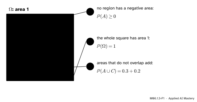
Draw the sample space \(\Omega\) as a square of area 1. Draw each event as a region inside it. Now read the probability of an event as the area of its region. Everything the rules of probability say is something you already believe about area.
M06.1.3-F1
Probability as area. The sample space is a square of area 1, and the probability of an event is the area of its region. The three numbered rules are the three axioms.
No area is negative. So no probability is negative.
The whole square has area 1. Something in \(\Omega\) always happens, so \({\Prob(\Omega) = 1}\).
Areas that do not overlap add up. If \(A\) and \(C\) are disjoint, the area of \({A \cup C}\) is the area of \(A\) plus the area of \(C\).
These three statements are the axioms of probability, proposed by Andrey Kolmogorov as the foundation of the subject. An axiom is a rule taken as the starting point and not proved. The next lesson derives every other rule you will use from these three, each with its own area picture.
Build it up
Step 1. A probability measures events, not just outcomes. We write \({\Prob(A)}\), read “the probability of \(A\)”, for the number given to the event \(A\). A single outcome \(\omega\) gets a probability through the event \({\{\omega\}}\) that holds only it.
Step 2. Three rules, nothing else. The three axioms say nothing about where the numbers come from: a fair coin, a loaded die, a model’s output or a hunch. Any assignment that obeys them is a probability, and every result that follows from the axioms holds for all of them at once. That is why one theory serves gambling, physics and machine learning.
Step 3. Two readings of the same number. People mean two things by “the probability of \(A\)”.
Long-run frequency. Repeat the experiment many times. The relative frequency of \(A\), the share of runs in which \(A\) occurs, settles down towards \({\Prob(A)}\) as the runs pile up.
Degree of belief. For a one-off event, such as “this email is spam” or “it rains tomorrow”, there is no long run. The probability is a measure of how strongly a person, or a model, expects the event, given what is known.
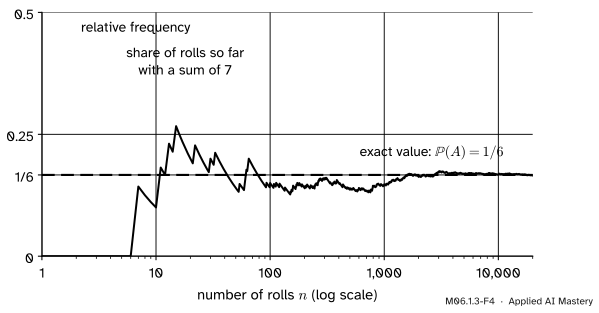
M06.1.3-F4
Two dice rolled 20,000 times in a simulation. The share of rolls with a sum of 7 swings widely at first and settles near the exact probability 1/6 as the rolls pile up.
Both readings obey the same three axioms, so the mathematics is the same whichever you prefer. The frequency reading is how we will check every exact answer in this course: compute it, then simulate. The belief reading is how a classifier’s output is used: there is only one email in front of you, and the model’s 0.7 is its degree of belief that this one is spam. Lesson M06.11.2 proves that relative frequencies settle down, as the picture suggests.
The formal statement
NoteDefinition: the axioms of probability
A probability on a sample space \(\Omega\) gives every event \(A\) a number \({\Prob(A)}\) such that
Axiom 1.\({\Prob(A) \geq 0}\) for every event \(A\).
Axiom 2.\({\Prob(\Omega) = 1}\).
Axiom 3. If \({A_1, A_2, A_3, \dots}\) are disjoint (no two share an outcome), then
Axiom 3 is stated for an endless sequence of events, because we need it for spaces like flips until the first head. It covers finitely many events too: for two disjoint events \(A\) and \(B\), use the sequence \({A, B, \emptyset, \emptyset, \dots}\). Its union is \({A \cup B}\), so \({\Prob(A \cup B)} = {\Prob(A)} + {\Prob(B)} + {\Prob(\emptyset)} + \cdots\). The next lesson proves from the axioms that \({\Prob(\emptyset) = 0}\), so the padding adds nothing and
\[
\begin{aligned}
&\Prob(A \cup B) = \Prob(A) + \Prob(B) \\
&\text{when } A \cap B = \emptyset .
\end{aligned}
\]
Finite sample spaces: add up the outcomes. Write \({p(\omega) = \Prob(\{\omega\})}\) for the probability of a single outcome. An event \(A\) is the union of the single-outcome events of its members, and these are disjoint, because a single-outcome event shares nothing with another. So Axiom 3 gives
\[
\Prob(A) = \sum_{\omega \in A} p(\omega) .
\]
The probabilities of the outcomes decide everything. Taking \({A = \Omega}\) and using Axiom 2, they must add up to 1. And the reverse holds: choose any numbers \({p(\omega) \geq 0}\) that add up to 1 over \(\Omega\), define \({\Prob(A)}\) by the sum above, and all three axioms hold. Axiom 1 holds because a sum of numbers that are not negative is not negative. Axiom 2 holds because the sum over all of \(\Omega\) is 1. Axiom 3 holds because each outcome of a union of disjoint events belongs to exactly one of them, so the sum over the union splits into one sum per event.
For a fair die, \({p(\omega) = \frac{1}{6}}\) for each face, so \({\Prob(\text{even}) = \frac{3}{6}}\). For two fair dice, each of the 36 outcomes gets \({\frac{1}{36}}\), so \({\Prob(\text{sum is } 7) = \frac{6}{36} = \frac{1}{6}}\).
A countably infinite space: flips until the first head. Number each outcome by the flip that brings the first head: outcome \(n\) is \({n - 1}\) tails followed by a head. A fair coin makes each of the \({2^n}\) ways that \(n\) flips can fall equally likely, and exactly one of them is outcome \(n\), so we give it \({p(n) = (\tfrac{1}{2})^n}\). Lessons M06.2.1 and M06.3.4 justify this step.
Is this a probability? Each \({p(n)}\) is positive, so Axiom 1 holds. For Axiom 2, add them all with the geometric sum of M01.7.3, \({a + ar + ar^2 + \cdots = \frac{a}{1 - r}}\) for \({-1 < r < 1}\), here with first term \({a = \frac{1}{2}}\) and ratio \({r = \frac{1}{2}}\):
An endless run of tails is not on the list. Had we added it as one more outcome, the listed outcomes would already use up the whole of the probability 1, so it could only get probability 0.
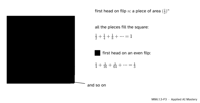
M06.1.3-F3
Flips until the first head as areas. Halving what is left again and again fills the square, so the probabilities add up to 1. The yellow pieces, a first head on an even flip, fill one third of it.
Now Axiom 3 does real work. “The first head comes on an even flip” is the union of the disjoint events \({\{2\}, \{4\}, \{6\}, \dots}\), so its probability is a geometric sum with first term \({\frac{1}{4}}\) and ratio \({\frac{1}{4}}\):
No finite rule could give this answer: the event holds infinitely many outcomes.
Go deeper: why adding in any order is safe
Axiom 3 lists the events in some order, but nothing says which order. For terms that are never negative, an endless sum has the same value in every order and in every grouping, a standard fact about series. That is what lets \({\Prob(A) = \sum_{\omega \in A} p(\omega)}\) make sense on a countably infinite space, and what lets us split the sum over a union into one sum per event. With negative terms it could fail; probabilities are never negative, so it never does.
Worked example
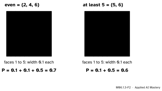
A die is loaded so that a six comes up half the time, and each other face a tenth of the time. Is this a probability? Find P(even) and P(at least 5).
Check the axioms. The outcome probabilities are \({p(1) = \cdots = p(5) = \frac{1}{10}}\) and \({p(6) = \frac{1}{2}}\). None is negative. They add to
For a fair die the same events have probabilities 0.5 and about 0.33. Same sample space, same events, different probabilities: the axioms fix the rules, not the numbers.
A proposal that fails. Suppose someone suggests \({\frac{1}{5}}\) for each of the faces 1 to 5 and \({\frac{1}{2}}\) for the six. Every number is positive, but they add to \({1 + \frac{1}{2} = 1.5}\), so \({\Prob(\Omega)}\) would be 1.5 and Axiom 2 fails. This is not a probability.
Code
Exact work first, with fractions.Fraction, so that no rounding hides a mistake.
from fractions import Fraction as Fp = {1: F(1, 10), 2: F(1, 10), 3: F(1, 10), 4: F(1, 10), 5: F(1, 10), 6: F(1, 2)}def prob(event):"""P(event) on a finite sample space: add up the outcomes."""returnsum(p[w] for w in event)print("each p >= 0:", all(v >=0for v in p.values()), " P(Omega) =", prob(p))print("P(even) =", prob({2, 4, 6}), " P(at least 5) =", prob({5, 6}))
each p >= 0: True   P(Omega) = 1
P(even) = 7/10   P(at least 5) = 3/5
The endless sums for flips until the first head cannot be added term by term, but their partial sums show the gap closing exactly as the geometric sum predicts.
total =sum(F(1, 2**n) for n inrange(1, 31)) # flips 1 to 30even =sum(F(1, 2**n) for n inrange(2, 31, 2)) # flips 2, 4, ..., 30print("all outcomes up to 30:", float(total), " missing:", 1- total)print("even flips up to 30:", float(even), " target 1/3")print("first head within 3 flips:", sum(F(1, 2**n) for n in (1, 2, 3)))
all outcomes up to 30: 0.9999999990686774   missing: 1/1073741824
even flips up to 30: 0.3333333330228925   target 1/3
first head within 3 flips: 7/8
Next the frequency reading: roll two dice many times in a simulation and watch the share of sums equal to 7. The shares printed below wander at first and end close to \({\frac{1}{6} \approx 0.167}\).
import numpy as nprng = np.random.default_rng(7)rolls = rng.integers(1, 7, size=(20_000, 2)) # high end excluded: faces 1 to 6is_seven = rolls.sum(axis=1) ==7share = np.cumsum(is_seven) / np.arange(1, len(is_seven) +1)for n in (10, 100, 1_000, 20_000):print(f"after {n:>6} rolls: {share[n -1]:.3f}")
after     10 rolls: 0.100
after    100 rolls: 0.150
after   1000 rolls: 0.147
after  20000 rolls: 0.165
Last, a classifier. A softmax layer turns three scores into three numbers that are positive and add to 1 (ML01.6.4). The classes are the outcomes, so these numbers satisfy the axioms, and the probability of “not class 3” is a sum.
softmax: [0.665 0.245 0.09 ]   total: 1.0
P(class 1 or class 2) = 0.91
Explore
The event explorer in lesson M06.1.4 gives every cell of the dice grid the probability \({\frac{1}{36}}\) and adds up the cells of any event you build, so you can test Axiom 3 on disjoint events and see what goes wrong on overlapping ones.
Pitfalls
M06.1.3-F5
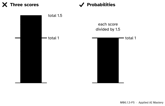
Wrong beside right. Three scores between 0 and 1 for three classes that exclude each other add to 1.5, which breaks Axiom 2. Divided by their total they become a probability.
“Any numbers between 0 and 1 are probabilities.”
Three separate yes-or-no detectors for cat, dog and bird might score one picture 0.7, 0.6 and 0.2. If every picture holds exactly one of the three, the classes are disjoint and cover \(\Omega\), so by Axioms 2 and 3 their probabilities must add to 1. These add to 1.5. Dividing by the total, or using a softmax, repairs it. Being between 0 and 1 is a consequence of the axioms, not a substitute.
“I rolled the dice ten times and got one 7, so the probability of a 7 is 0.1.”
That is a relative frequency from a short run, and short runs swing widely, as the left end of the frequency chart shows. The probability is the value the share settles towards over a long run (or the value given by the axioms and a model of fair dice, \({\frac{1}{6}}\)). Ten rolls are evidence about it, not a measurement of it.
“Axiom 3 lets me add the probabilities of any two events.”
Only of disjoint ones. “The sum is 7” has probability \({\frac{6}{36}}\) and “the first die is even” has \({\frac{18}{36}}\), but the chance of one or the other is not \({\frac{24}{36}}\): three outcomes lie in both and would be counted twice. The next lesson finds the right answer, \({\frac{21}{36}}\).
Check yourself
Recall
1. State the three axioms of probability.
Show answer
\({\Prob(A) \geq 0}\) for every event; \({\Prob(\Omega) = 1}\); and for disjoint events \({A_1, A_2, \dots}\) the probability of their union is the sum of their probabilities.
2. On a finite sample space, how do you find the probability of an event?
Show answer
Add the probabilities of its outcomes: \({\Prob(A) = \sum_{\omega \in A} p(\omega)}\).
3. What must be true of numbers \({p(\omega)}\) for them to define a probability on a finite \(\Omega\)?
Show answer
None may be negative, and together they must add up to 1.
4. What are the two readings of a probability?
Show answer
Long-run frequency: the share of many repeated runs in which the event occurs settles towards it. Degree of belief: how strongly someone, or a model, expects a one-off event.
5. A coin is flipped until the first head. What is the probability that the first head comes on an even flip?
Show answer
\(\frac{1}{4} + \frac{1}{16} + \cdots = \frac{1/4}{1 - 1/4} = \frac{1}{3}\), by Axiom 3 and the geometric sum.
Exercises
1.★ On \({\Omega = \{a, b, c\}}\), which of these assignments \({(p(a), p(b), p(c))}\) are probabilities? (i) \({(0.5, 0.3, 0.2)}\) (ii) \({(0.6, 0.6, -0.2)}\) (iii) \({(0.3, 0.3, 0.3)}\).
Show solution
(i) Yes: all are at least 0 and they add to 1. (ii) No: they add to 1, but \({-0.2}\) breaks Axiom 1. (iii) No: they add to 0.9, so \({\Prob(\Omega) = 0.9}\) breaks Axiom 2.
2.★★ A die is loaded so that each face comes up with probability proportional to its number: \({p(k) = ck}\) for \({k = 1, \dots, 6}\). Find \(c\), then P(even).
Show solution
Axiom 2 needs \({c(1 + 2 + \cdots + 6) = 21c = 1}\), so \({c = \frac{1}{21}}\). Then
3.★★★ A coin shows heads with probability \(q\), where \({0 < q \leq 1}\), and is flipped until the first head. Outcome \(n\) is given \({p(n) = (1 - q)^{n - 1} q}\). Show that these add up to 1, and find the probability that at least three flips are needed when \({q = \frac{1}{3}}\).
Show solution
The sum is geometric with first term \({a = q}\) and ratio \({r = 1 - q}\), and \({0 \leq r < 1}\), so
“At least three flips” is the union of the disjoint outcomes \({3, 4, 5, \dots}\), a geometric sum with first term \({(1 - q)^2 q}\) and the same ratio:
Charles M. Grinstead and J. Laurie Snell, Introduction to Probability, second edition (free PDF). Section 1.2: Definition 1.2 (outcome probabilities that are not negative and add to 1, with \({\Prob(E)}\) as a sum over \(E\)) and Theorem 1.1 (the properties that follow). Example 1.13: a coin tossed until the first head, \({m(n) = 1/2^n}\), summing to 1 by the geometric series, with probability \({\frac{1}{3}}\) for an even number of tosses.
Jeremy Orloff and Jonathan Bloom, Reading 2: Probability, terminology and examples, MIT OpenCourseWare 18.05, Spring 2022. Section 2.4: the probability function and \({\Prob(E) = \sum_{\omega \in E} \Prob(\omega)}\); Example 7, flip until heads.
Marc Peter Deisenroth, A. Aldo Faisal and Cheng Soon Ong, Mathematics for Machine Learning (free PDF). Section 6.1.1: the Bayesian (degree of belief) and frequentist (relative frequency in the limit) readings of probability. Section 6.1.2: Kolmogorov’s axioms behind the probability space.