A deliberately PyTorch-shaped library on top of the engine: Parameter, Module with a recursive parameters(), Linear, ReLU, Sequential and an SGD optimizer, with why gradients must be zeroed and why updates happen outside the graph.
DL01.6.3L2 Intermediate25 minIn review (what this means)
The maths and code on this page are checked by automated tests on every change, but an independent reader has not signed it off yet. Spot a mistake or a confusing step? Tell us.
Explain what a Parameter, a Module, parameters() and an optimizer are, and how they share the same tensor objects.
Implement Linear with its weight stored as (out, in), ReLU, Sequential and SGD with zero_grad() and step() in under a hundred lines.
Count the parameters of a multilayer perceptron from its layer sizes, and check the count of a 2-16-16-2 network.
Explain why gradients accumulate and must be zeroed between steps, and why the update must happen outside the graph.
The question
Every PyTorch training script has the same few lines: build model from layers, hand model.parameters() to an optimizer, then repeat optimizer.zero_grad(), loss.backward(), optimizer.step(). The engine of this module can already do backward. What are the objects around it, how does an optimizer find all the weights of a deep network, and what goes wrong if you leave out zero_grad?
From the last lesson
1. In the course convention \({Z = XW\T + \vect{1}\vect{b}\T}\), what are the gradients of \(W\) and \(\vect{b}\)?
Show answer
\({G\T X}\), shape (out, in), and the column sums of \(G\), shape (out,).
2. What is the backward rule of broadcasting?
Show answer
Sum the gradient over every axis that was stretched or added in front, so that it ends with the shape of the array.
Intuition
A network is a tree of parts. The root holds the layers, a layer holds its weight and bias, and the weight and bias are tensors the training is allowed to change. Walk the tree and collect those tensors, and you have a list the optimizer can update.
DL01.6.3-F1
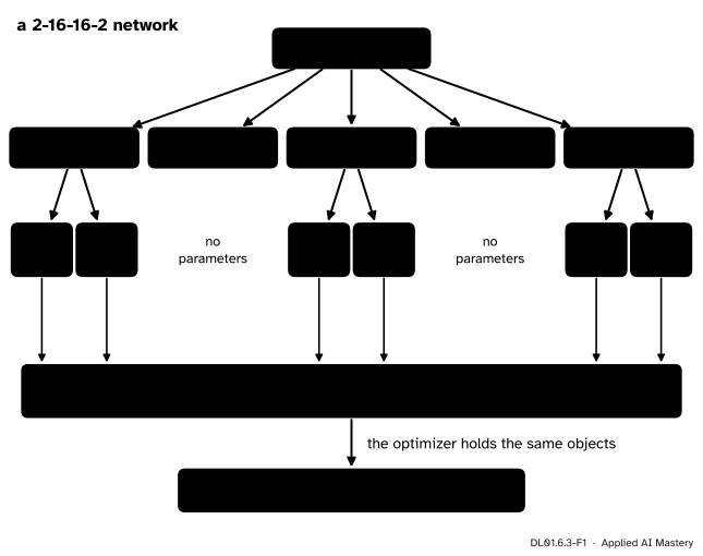
The library of this lesson, drawn as the tree it builds. parameters() walks the tree and returns the six tensors marked for learning. The optimizer keeps references to those same objects, so when it changes them, the network changes.
Nothing is copied. The optimizer’s list and the layers point at the same six objects, which is why step() can update the network without knowing anything about its layers.
Build it up
Step 1. A Parameter is a Tensor with a mark on it. It behaves exactly like a tensor; its type says “the training may change me”. A layer’s weight and bias are Parameters. Its inputs and its intermediate results are plain tensors.
Step 2. A Module holds Parameters and other Modules. Its parameters() method looks through its own attributes: a Parameter is collected, a Module is asked for its parameters in turn, and a list of Modules is searched item by item. That recursion is what lets the optimizer find the weights of a network of any depth.
Step 3. Linear, ReLU, Sequential.Linear(n_in, n_out) stores a weight of shape (n_out, n_in), the shape PyTorch’s nn.Linear uses, and a bias of shape (n_out,), and computes x @ W.T + b. ReLU has no parameters. Sequential calls its layers in order.
DL01.6.3-F2
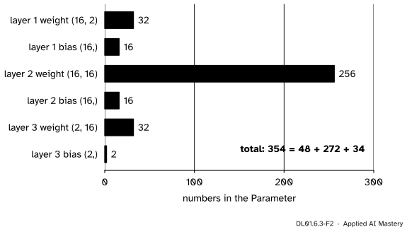
Where the 354 numbers of a 2-16-16-2 network live. The square hidden-to-hidden weight holds more than the rest put together.
Step 4. An optimizer holds the list and does two things.zero_grad() sets every parameter’s grad to zero. step() moves every parameter against its gradient, \({w \leftarrow w - \eta\,\nabla_w L}\), the gradient descent of ML01.5.
The formal statement
NoteThe parameter count and the update
A layer from \(n_{l-1}\) inputs to \(n_l\) outputs has a weight of shape \({(n_l, n_{l-1})}\) and a bias of shape \({(n_l,)}\), so \({n_l(n_{l-1} + 1)}\) parameters. A network with widths \({n_0, \dots, n_D}\) has
\[
\sum_{l=1}^{D} n_l\,(n_{l-1} + 1)
\]
parameters. One step of SGD with learning rate \(\eta\) replaces every parameter \(\theta\) by \({\theta} - {\eta\,\cgrad{\nabla_\theta L}}\), using the gradients of the current mini-batch only.
For the 2-16-16-2 network the sum is \({16 \cdot 3} + {16 \cdot 17} + {2 \cdot 17} = {48} + {272} + {34} = {354}\).
Why the gradients accumulate. In DL01.6.1 the leaves of the graph keep what their grad holds, and every closure adds with +=. This is by design. A weight used twice in one forward pass, a shared weight, must collect both contributions (M05.8.3, DL01.5.3), and adding is the only way to do that when the contributions arrive one closure at a time. The same rule means that a second call of backward adds a second gradient on top of the first. PyTorch documents the same behaviour: backward accumulates in the leaves, and you may need to zero .grad first.
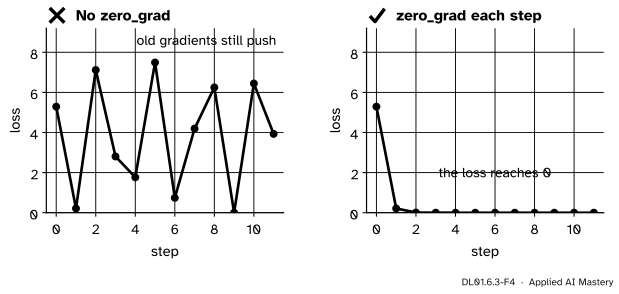
So the loop must clear the gradients before each backward pass. If it does not, step \(t\) uses the sum of all the gradients so far:
Old gradients, computed at old parameters, keep pushing after they have stopped being true.
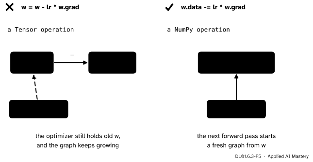
Why the update happens outside the graph. Written with tensor operations, w = w - lr * w.grad makes a new tensor whose parents are the old w and a constant. The name w now points at a result, not a Parameter, the optimizer still holds the old object, and every later forward pass would build its graph through a growing chain of past updates. The update is not part of the function being differentiated, so it is done on the arrays: w.data -= lr * w.grad changes the numbers inside the same object.
DL01.6.3-F5
The update is not part of the model. Done with tensor operations it adds nodes to a graph and breaks the link between the optimizer and the network; done on .data it does neither.
The same idea gives a switch, no_grad(): inside it, operations compute their data but record no parents and no closure. An evaluation pass that will never be differentiated then builds no graph and keeps no arrays alive for a backward pass that never comes.
Worked example
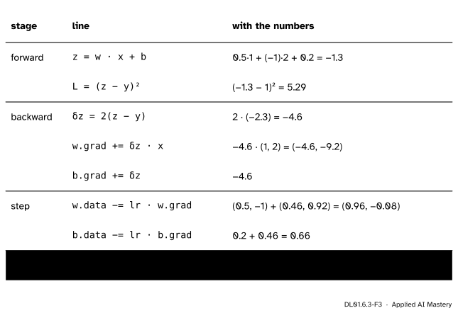
One step of a tiny layer. Take Linear(2, 1) with weight \({(0.5, -1)}\) and bias 0.2, one example \({\vect{x} = (1, 2)}\) with target \({y = 1}\), the squared error and \({\eta = 0.1}\).
DL01.6.3-F3
Forward, backward and one SGD step, with every number. The loss falls from 5.29 to 0.2116.
Now the second step. Zeroed first, the new gradient is \({2 \times 0.46 \times (1, 2)} = {(0.92, 1.84)}\) for \(w\) and 0.92 for \(b\), and the step brings \(z\) to 0.908 and the loss to about 0.0085. Not zeroed, the grads hold \({(-4.6, -9.2)} + {(0.92, 1.84)} = {(-3.68, -7.36)}\) and \({-3.68}\): the old gradient still points up, so \(z\) shoots to 3.668 and the loss to about 7.12.
Code
The engine of DL01.6.1 and DL01.6.2, gathered into one class, is folded here.
The engine of DL01.6.1 and DL01.6.2
import numpy as npclass Tensor:def__init__(self, data):self.data = np.asarray(data, dtype=float)self.grad = np.zeros_like(self.data)self.parents = ()self.backward_fn =Nonedef record(self, parents, backward_fn):self.parents, self.backward_fn = parents, backward_fnreturnself@propertydef shape(self):returnself.data.shapedef__add__(self, other): other = lift(other) out = Tensor(self.data + other.data)def backward_fn():self.grad += unbroadcast(out.grad, self.shape) other.grad += unbroadcast(out.grad, other.shape)return out.record((self, other), backward_fn)def__sub__(self, other): other = lift(other) out = Tensor(self.data - other.data)def backward_fn():self.grad += unbroadcast(out.grad, self.shape) other.grad += unbroadcast(-out.grad, other.shape)return out.record((self, other), backward_fn)def__mul__(self, other): other = lift(other) out = Tensor(self.data * other.data)def backward_fn():self.grad += unbroadcast(other.data * out.grad, self.shape) other.grad += unbroadcast(self.data * out.grad, other.shape)return out.record((self, other), backward_fn)__radd__, __rmul__=__add__, __mul__def__neg__(self): out = Tensor(-self.data)def backward_fn():self.grad +=-out.gradreturn out.record((self,), backward_fn)def__pow__(self, k): out = Tensor(self.data ** k)def backward_fn():self.grad += k *self.data ** (k -1) * out.gradreturn out.record((self,), backward_fn)def exp(self): out = Tensor(np.exp(self.data))def backward_fn():self.grad += out.data * out.gradreturn out.record((self,), backward_fn)def log(self): out = Tensor(np.log(self.data))def backward_fn():self.grad += out.grad /self.datareturn out.record((self,), backward_fn)def tanh(self): out = Tensor(np.tanh(self.data))def backward_fn():self.grad += (1- out.data **2) * out.gradreturn out.record((self,), backward_fn)def relu(self): out = Tensor(np.maximum(self.data, 0))def backward_fn():self.grad += (self.data >0) * out.gradreturn out.record((self,), backward_fn)def__matmul__(self, other): out = Tensor(self.data @ other.data)def backward_fn():self.grad += out.grad @ other.data.T other.grad +=self.data.T @ out.gradreturn out.record((self, other), backward_fn)defsum(self, axis=None, keepdims=False): out = Tensor(self.data.sum(axis=axis, keepdims=keepdims))def backward_fn(): g = out.grad if keepdims or axis isNoneelse np.expand_dims(out.grad, axis)self.grad += np.broadcast_to(g, self.shape)return out.record((self,), backward_fn)def mean(self, axis=None, keepdims=False): total =self.sum(axis=axis, keepdims=keepdims)return total * (total.data.size /self.data.size)@propertydef T(self): out = Tensor(self.data.T)def backward_fn():self.grad += out.grad.Treturn out.record((self,), backward_fn)def topo_order(self): order, seen, stack = [], set(), [(self, False)]while stack: node, finished = stack.pop()if finished: order.append(node)elifid(node) notin seen: seen.add(id(node)) stack.append((node, True)) stack.extend((p, False) for p in node.parents ifid(p) notin seen)return orderdef backward(self): order =self.topo_order()for node in order:if node.parents: node.grad = np.zeros_like(node.data)self.grad = np.ones_like(self.data)for node inreversed(order):if node.backward_fn: node.backward_fn()def lift(x):return x ifisinstance(x, Tensor) else Tensor(x)def unbroadcast(grad, shape):while grad.ndim >len(shape): grad = grad.sum(axis=0)for axis, size inenumerate(shape):if size ==1and grad.shape[axis] !=1: grad = grad.sum(axis=axis, keepdims=True)return graddef cross_entropy(z, labels): n = z.shape[0] shifted = z.data - z.data.max(axis=1, keepdims=True) log_p = shifted - np.log(np.exp(shifted).sum(axis=1, keepdims=True)) out = Tensor(-log_p[np.arange(n), labels].mean())def backward_fn(): g = np.exp(log_p) g[np.arange(n), labels] -=1 z.grad += g / n * out.gradreturn out.record((z,), backward_fn)
First the switch. record is the one place where an operation attaches its parents and closure, so the switch lives there.
import contextlibTensor.recording =Truedef record(self, parents, backward_fn):if Tensor.recording: # under no_grad: data only, no graphself.parents, self.backward_fn = parents, backward_fnreturnselfTensor.record = record@contextlib.contextmanagerdef no_grad(): Tensor.recording =Falsetry:yieldfinally: Tensor.recording =True
The library itself.
class Parameter(Tensor):"""A Tensor that the optimizer is allowed to change."""class Module:def parameters(self):"""Every Parameter in this module and, recursively, in the modules it holds.""" found = []for value invars(self).values():for item in (value ifisinstance(value, list) else [value]):ifisinstance(item, Parameter): found.append(item)elifisinstance(item, Module): found.extend(item.parameters())return founddef__call__(self, x):returnself.forward(x)class Linear(Module):def__init__(self, n_in, n_out, rng): bound =1/ np.sqrt(n_in) # PyTorch's range for nn.Linear; DL02.3 explainsself.weight = Parameter(rng.uniform(-bound, bound, size=(n_out, n_in)))self.bias = Parameter(rng.uniform(-bound, bound, size=n_out))def forward(self, x):return x @self.weight.T +self.biasclass ReLU(Module):def forward(self, x):return x.relu()class Sequential(Module):def__init__(self, *layers):self.layers =list(layers)def forward(self, x):for layer inself.layers: x = layer(x)return xclass SGD:def__init__(self, params, lr):self.params, self.lr =list(params), lrdef zero_grad(self):for p inself.params: p.grad = np.zeros_like(p.data)def step(self):for p inself.params: p.data -=self.lr * p.grad # on the array: outside the graph
A 2-16-16-2 network, its parameters, and a forward pass on four points:
rng = np.random.default_rng(0)model = Sequential(Linear(2, 16, rng), ReLU(), Linear(16, 16, rng), ReLU(), Linear(16, 2, rng))params = model.parameters()print("shapes:", [p.shape for p in params])print("parameters:", sum(p.data.size for p in params))x = Tensor(rng.normal(size=(4, 2)))print("logits shape:", model(x).shape)
nodes recorded: 18  under no_grad: 1
same numbers: True
The recorded pass has 18 nodes: the input, the six Parameters, and eleven results, three for each Linear (the transpose, the product and the addition of the bias) and one for each ReLU. Under no_grad the output is a lone tensor with no parents.
Explore
The module’s interactive, Broadcast and backward, is in DL01.6.2. Try the bias case there, shapes (2, 3) and (1, 3): it is the addition inside every Linear.
Pitfalls
DL01.6.3-F4
Wrong beside right, on the worked example. Without zero_grad, each step uses the sum of every gradient so far, and the loss jumps about instead of settling.
“backward replaces the old gradient.”
It adds to it. The engine, like PyTorch, accumulates in the leaves so that shared weights work, and the price is that the training loop must call zero_grad() before each backward pass. The bug is quiet: the loss still moves, just badly.
“w = w - lr * w.grad is the update.”
On tensors it makes a new node with parents. The optimizer keeps the old Parameter, so the model no longer changes, and the graph grows by a node per step. Update the array in place, w.data -= lr * w.grad, outside the graph.
“A layer’s weight has shape (in, out).”
In this library and in PyTorch it is (out, in), and the layer computes x @ W.T + b. Copying weights between a library that stores (in, out), such as scikit-learn’s coefs_, and one that stores (out, in) needs a transpose. With equal sizes in and out the shapes match either way, so the mistake can pass every shape check.
Check yourself
Recall
1. What does parameters() return, and how does it find the weights of a deep network?
Show answer
The list of every Parameter in the module and in the modules it holds; it looks through its attributes and asks each Module it finds for its own parameters, recursively.
2. How many parameters does a layer from \(n_{l-1}\) inputs to \(n_l\) outputs have?
Show answer
\({n_l(n_{l-1} + 1)}\): a weight of shape \({(n_l, n_{l-1})}\) and \(n_l\) biases.
3. Why do gradients accumulate across calls of backward?
Show answer
Closures add into grad and leaves keep their grad, which is what a weight used more than once needs; so a second backward pass adds to the first.
4. Why is the update done on .data instead of with tensor operations?
Show answer
The update is not part of the function being differentiated. With tensor operations it would create a new node with parents, leave the optimizer holding the old Parameter and grow the graph.
5. What does no_grad() change?
Show answer
Operations still compute their data but record no parents and no closure, so no graph is built.
Exercises
1.★ Count the parameters of a 64-32-10 network, the course’s image classifier.
2.★★ Continue the worked example for one more step without zero_grad and confirm the loss of about 7.12.
Show solution
After step 1, \({w = (0.96, -0.08)}\), \({b = 0.66}\) and \({z = 1.46}\). Step 2’s own gradient is \({\delta_z = 2(1.46 - 1) = 0.92}\), so it adds \({(0.92, 1.84)}\) and 0.92 to grads that still hold \({(-4.6, -9.2)}\) and \({-4.6}\): totals \({(-3.68, -7.36)}\) and \({-3.68}\). The step gives \({w} = {(0.96 + 0.368,\ -0.08 + 0.736)} = {(1.328, 0.656)}\) and \({b = 0.66 + 0.368 = 1.028}\), so \({z = 1.328 + 1.312 + 1.028 = 3.668}\) and \({L = 2.668^2 \approx 7.118}\).
3.★★★ A weight matrix is shared: the same Parameter is used by two Linear layers in one forward pass. Explain why parameters() of a Sequential holding both layers lists it twice, what SGD.step() would then do, and how to fix it.
Show solution
parameters() collects each layer’s attributes, and both layers hold the same object, so it appears twice in the list. During backward its grad correctly collects both contributions, by accumulation. But step() walks the list and subtracts \({\eta\,\nabla}\) once per entry, so the shared weight moves twice as far as it should. The fix is to remove repeats by identity: keep a set of id(p) already seen and skip any parameter found again. PyTorch’s named_parameters does this by default (remove_duplicate=True).
Summary card
A library is a tree of Modules whose Parameters the optimizer holds.
DL01.6.3-F1
Walk the tree, collect, update.
Parameters per layer: \({n_l(n_{l-1} + 1)}\); 354 for 2-16-16-2.
Linear: weight (out, in), computes x @ W.T + b.
Each step: zero_grad(), backward(), step().
Update on .data; evaluate under no_grad().
Sources and next steps
Sources. Each was opened and checked against this lesson on 15 November 2026.
PyTorch 2.15, torch.nn.Linear: computes \({y = xA\T + b}\), with weight of shape (out_features, in_features) and bias of shape (out_features), both initialised from \({\mathcal{U}(-\sqrt{k}, \sqrt{k})}\) with \({k = 1/\text{in\_features}}\).
PyTorch 2.15, torch.Tensor.backward: the function accumulates gradients in the leaves, so .grad may need zeroing first; and Autograd mechanics: computations in no-grad mode behave as if no input requires a gradient and are not recorded; and torch.nn.Module: named_parameters removes duplicated parameters by default.
A. Karpathy, micrograd (MIT licence): a small neural network library with a PyTorch-like API on top of a scalar engine, trained with two hidden layers of 16 units on the moons; the design this lesson follows on arrays.
I. Goodfellow, Y. Bengio and A. Courville, Deep Learning, section 6.5.8: real implementations add each contribution into a single buffer instead of computing every term separately and summing at the end.