import numpy as np

class Tensor:
    """A NumPy array that remembers how it was made, so that gradients can flow back through it."""
    def __init__(self, data):
        self.data = np.asarray(data, dtype=float)
        self.grad = np.zeros_like(self.data)     # d(output)/d(entry), same shape as data
        self.parents = ()                        # the tensors this one was computed from
        self.backward_fn = None                  # passes self.grad back to the parents

    def record(self, parents, backward_fn):
        self.parents, self.backward_fn = parents, backward_fn
        return self

    @property
    def shape(self):
        return self.data.shape

    def __add__(self, other):
        assert self.shape == other.shape, "same shapes only, until DL01.6.2"
        out = Tensor(self.data + other.data)
        def backward_fn():
            self.grad += out.grad
            other.grad += out.grad
        return out.record((self, other), backward_fn)

    def __sub__(self, other):
        assert self.shape == other.shape, "same shapes only, until DL01.6.2"
        out = Tensor(self.data - other.data)
        def backward_fn():
            self.grad += out.grad
            other.grad += -out.grad
        return out.record((self, other), backward_fn)

    def __mul__(self, other):
        assert self.shape == other.shape, "same shapes only, until DL01.6.2"
        out = Tensor(self.data * other.data)
        def backward_fn():
            self.grad += other.data * out.grad
            other.grad += self.data * out.grad
        return out.record((self, other), backward_fn)

    def __neg__(self):
        out = Tensor(-self.data)
        def backward_fn():
            self.grad += -out.grad
        return out.record((self,), backward_fn)

    def __pow__(self, k):                        # k is a plain number
        out = Tensor(self.data ** k)
        def backward_fn():
            self.grad += k * self.data ** (k - 1) * out.grad
        return out.record((self,), backward_fn)

    def exp(self):
        out = Tensor(np.exp(self.data))
        def backward_fn():
            self.grad += out.data * out.grad     # the slope of exp is exp: reuse it
        return out.record((self,), backward_fn)

    def log(self):
        out = Tensor(np.log(self.data))
        def backward_fn():
            self.grad += out.grad / self.data
        return out.record((self,), backward_fn)

    def sin(self):
        out = Tensor(np.sin(self.data))
        def backward_fn():
            self.grad += np.cos(self.data) * out.grad
        return out.record((self,), backward_fn)

    def tanh(self):
        out = Tensor(np.tanh(self.data))
        def backward_fn():
            self.grad += (1 - out.data ** 2) * out.grad
        return out.record((self,), backward_fn)

    def relu(self):
        out = Tensor(np.maximum(self.data, 0))
        def backward_fn():
            self.grad += (self.data > 0) * out.grad   # slope 0 at exactly 0
        return out.record((self,), backward_fn)

    def topo_order(self):
        """Every tensor this one depends on, each listed after its parents."""
        order, seen, stack = [], set(), [(self, False)]
        while stack:
            node, finished = stack.pop()
            if finished:
                order.append(node)
            elif id(node) not in seen:
                seen.add(id(node))
                stack.append((node, True))
                stack.extend((p, False) for p in node.parents if id(p) not in seen)
        return order

    def backward(self):
        order = self.topo_order()
        for node in order:
            if node.parents:                     # results start from zero; leaves keep their grad
                node.grad = np.zeros_like(node.data)
        self.grad = np.ones_like(self.data)      # the seed
        for node in reversed(order):             # children before parents
            if node.backward_fn:
node.backward_fn()From scalars to tensors
Rebuild the scalar Var class of M05.8 as a Tensor class around a NumPy array: data, grad, parents and a backward closure recorded as each operation runs, with a vector-Jacobian product for every elementwise operation.
Before this lesson: M05.8 Computational graphs and automatic differentiation M05.9 Backpropagation as reverse-mode differentiation DL01.5 Backpropagation by hand
What you will be able to do
- Describe a Tensor as a NumPy array together with a gradient of the same shape, the tensors it was made from and a backward closure recorded when the operation ran.
- Derive the vector-Jacobian product of an elementwise operation and explain why it never needs the Jacobian matrix.
- Implement add, subtract, multiply, negate, power, exp, log, sin, tanh and ReLU with their backward closures, and a backward method that sorts the graph topologically.
- Check the engine on the running program of M05.8 run elementwise on arrays, against the hand formulas and against central differences.
The question
The Var class of M05.8.3 differentiated \({\ln x_1 + x_1 x_2 - \sin x_2}\) at one point with a few lines of Python. A hidden layer of 100 units with 100 inputs, on a batch of 64 examples, makes 6,400 numbers at once, and its matrix product needs 640,000 multiplications. Wrapped one number at a time, every one of those would be a Python object on the tape. What must change so that the same few lines of backward logic work on whole arrays at once?
Intuition
Keep the graph and change what sits at each node. In M05.8 a node held one number and its adjoint. Here a node holds a whole NumPy array, the data, and a second array of the same shape, the grad, which will hold the derivative of the output with respect to every entry.
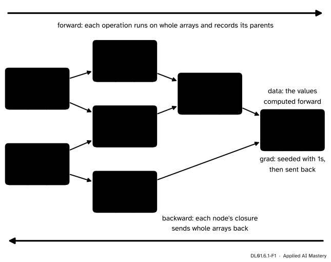
The running program of M05.8, now run on arrays of three numbers. Every node keeps its values (top row) and its gradient (bottom row, green). The first column is the point \({(2, 5)}\) of M05.8, and its gradients 5.5 and 1.72 are the ones found there.
Look at the bottom-left corner. The first column repeats M05.8: \({(5.5,\ 1.716)}\). The other two columns are two more points of the same program, differentiated in the same sweep. The graph still has seven nodes. With arrays of a million entries it would still have seven, and each node’s work would be one NumPy call on a whole array. That is the whole idea of a tensor engine: the graph is as small as the program, not as large as the data.
Build it up
Step 1. A tensor is a record of four things. The data, the grad (zeros to begin with), the parents it was computed from, and a backward closure: a small function, written at the moment the operation ran, that knows how to pass this tensor’s grad back to its parents.
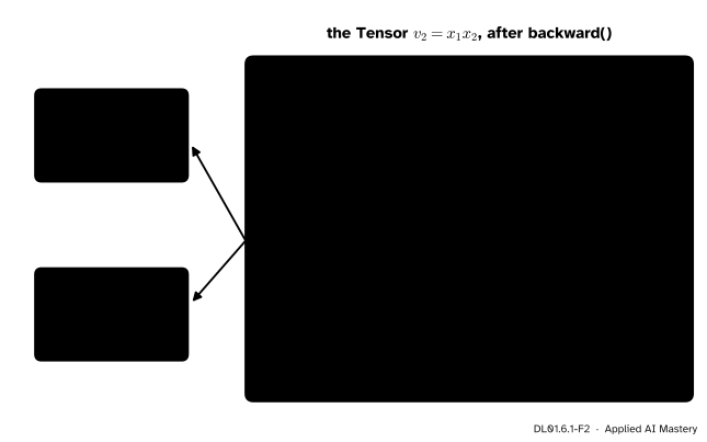
One tensor of the running program, opened up. The closure refers to the arrays of the parents and to the tensor’s own grad, so it can run long after the product was computed.
Step 2. An operation computes and records. Running \({v_2 = x_1 x_2}\) does two things: NumPy computes the product, and the result is given its parents and its closure. So the graph is built by the program as it runs, one node per operation. This is called define-by-run, and it is how PyTorch and Karpathy’s micrograd work.
Step 3. The backward rule of an elementwise operation is an elementwise product. Entry \(i\) of \({\sin x_2}\) depends on entry \(i\) of \(x_2\) only. So the Jacobian is diagonal, and multiplying by it is the same as multiplying entry by entry.
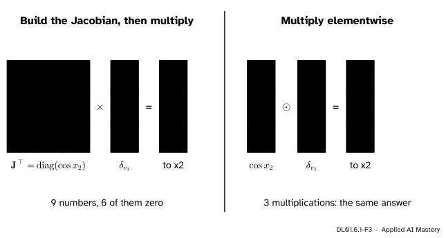
The backward step of \({v_3 = \sin x_2}\) in the running program. Writing out the Jacobian wastes \(n^2\) numbers, almost all zero. The elementwise product gives the same column with \(n\) multiplications.
Step 4. Backward sorts, seeds and sweeps. The output’s grad is set to ones. The graph is put in topological order, every node after its parents, and the closures are called from the end of that list to the start, each adding into its parents’ grads. A node is reached only after all of its children have reported, the rule M05.8.3 needed for a value used twice.
The formal statement
Derivation. The first line is the adjoint recurrence of M05.8.3 written for a whole array at once: the adjoint of entry \(u_j\) collects \({\delta_{v_i}\,\partial v_i / \partial u_j}\) from every entry \(v_i\) that uses it, and
\[ \sum_i \pd{v_i}{u_j}\,\delta_{v_i} = \big(\mat{J}_f\T\vect{\delta}_{\vect{v}}\big)_j , \]
since \({\partial v_i / \partial u_j}\) is entry \((i, j)\) of the Jacobian. For an elementwise operation, \(v_i\) depends on \(u_i\) alone, so \({\partial v_i/\partial u_j} = {g'(u_i)}\) when \({i = j}\) and 0 otherwise. The sum then has one term, \({g'(u_j)\,\delta_{v_j}}\), which is the second line.
An operation of two arguments has one rule for each. For \({\vect{v}} = {\vect{a} \odot \vect{b}}\), entry \(v_i = a_i b_i\) has slope \(b_i\) in \(a_i\) and \(a_i\) in \(b_i\), so it sends \({\vect{b} \odot \vect{\delta}_{\vect{v}}}\) to \(\vect{a}\) and \({\vect{a} \odot \vect{\delta}_{\vect{v}}}\) to \(\vect{b}\). Applied to each operation in turn:
| Operation | Sent back to the input |
|---|---|
| \({a + b}\), \({a - b}\) | \(\delta\) to \(a\); \(\delta\) or \(-\delta\) to \(b\) |
| \({a \odot b}\) | \({b \odot \delta}\) to \(a\), \({a \odot \delta}\) to \(b\) |
| \({-a}\), \({a^k}\) | \(-\delta\); \({k\,a^{k-1} \odot \delta}\) |
| \({e^{a}}\), \({\ln a}\) | \({e^{a} \odot \delta}\); \({\delta / a}\) |
| \({\sin a}\), \({\tanh a}\) | \({\cos a \odot \delta}\); \({(1 - \tanh^2 a) \odot \delta}\) |
| \({\operatorname{relu} a}\) | \(\delta\) where \({a > 0}\), else 0 |
Two of these reuse the forward result instead of recomputing it: \({e^a}\) is the output itself, and so is \(\tanh a\). At \({a = 0}\) ReLU has no derivative; PyTorch’s autograd notes ask for the subgradient of smallest size there, which is 0, and the engine follows it.
Seeding with ones. If the output \(\vect{y}\) is an array, the seed \({\vect{\delta}_{\vect{y}} = \vect{1}}\) makes the sweep return \({\mat{J}\T\vect{1}}\): the gradient of \({\sum_i y_i}\). For an elementwise program each \(y_i\) depends only on entry \(i\) of the inputs, so this is every entry’s own derivative. A training loss is a single number, and there the seed is the usual 1.
Go deeper: why the depth-first sort puts every node after its parents
The sort pops a node, marks it seen, pushes a “finished” marker for it, and then pushes its unseen parents above the marker. The stack is last in, first out, so every parent, and everything above it, is finished before the marker is popped, and a node is appended only when its marker is popped. Could a parent already be seen but not finished? Then the node would lie above that parent’s marker, so it would have been reached from the parent by following parents, making it an ancestor of its own parent: a cycle. A program that only ever computes new values from old ones has no cycles, so every node lands in the list after all its parents, and reversing the list puts every node before its parents.
Worked example
The running program on three points. Take \({x_1 = (2, 1, 0.5)}\) and \({x_2 = (5, 0, 2)}\). The forward pass gives \({v_1 = \ln x_1}\), \({v_2 = x_1 \odot x_2 = (10, 0, 1)}\), \({v_3 = \sin x_2}\), \({v_4 = v_1 + v_2}\) and \({y} = {v_4} - {v_3} \approx {(11.652,\ 0,\ -0.602)}\). Now the closures run in reverse topological order.
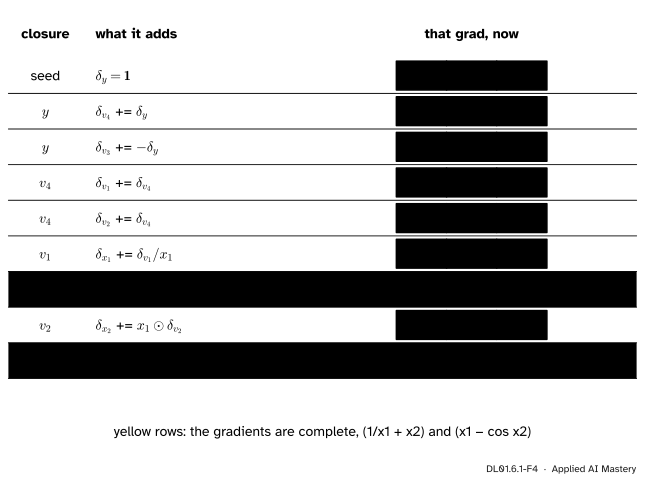
The backward sweep in the order the engine runs it. Each input collects two contributions, one per use. The yellow rows finish the gradient of each input.
- Seed: \({\delta_y = (1, 1, 1)}\).
- The closure of \({y = v_4 - v_3}\) adds \(\delta_y\) to \(v_4\) and \({-\delta_y}\) to \(v_3\).
- The closure of \({v_4 = v_1 + v_2}\) copies \({(1, 1, 1)}\) to both.
- The closure of \({v_1 = \ln x_1}\) adds \({\delta_{v_1} / x_1} = {(0.5,\ 1,\ 2)}\) to \(x_1\).
- The closure of \(v_2\) adds \({x_2 \odot \delta_{v_2}} = {(5,\ 0,\ 2)}\) to \(x_1\), which now holds \({(5.5,\ 1,\ 4)}\), and \({x_1 \odot \delta_{v_2}} = {(2,\ 1,\ 0.5)}\) to \(x_2\).
- The closure of \({v_3 = \sin x_2}\) adds \({\cos x_2 \odot (-1, -1, -1)}\), about \({(-0.284,\ -1,\ 0.416)}\), to \(x_2\), which now holds about \({(1.716,\ 0,\ 0.916)}\).
The hand formulas agree: \({\partial y / \partial x_1} = {1/x_1} + {x_2}\) gives \({(5.5, 1, 4)}\), and \({\partial y / \partial x_2} = {x_1} - {\cos x_2}\) gives \({(1.716, 0, 0.916)}\) to three decimals.
Code
The class, from scratch. Every operation computes its data with NumPy, then calls record to attach its parents and its closure. For now both arguments of an operation must have the same shape; DL01.6.2 lifts that restriction.
The running program, run once on three points:
x1 = Tensor([2.0, 1.0, 0.5])
x2 = Tensor([5.0, 0.0, 2.0])
y = x1.log() + x1 * x2 - x2.sin()
y.backward()
print("y       =", np.round(y.data, 3))
print("x1.grad =", np.round(x1.grad, 3))
print("x2.grad =", np.round(x2.grad, 3))
print("nodes in the graph:", len(y.topo_order()))
y = [11.652 0. -0.602]
x1.grad = [5.5 1. 4. ]
x2.grad = [1.716 0. 0.916]
nodes in the graph: 7The first entries repeat M05.8.3. Now a sterner test: a program that uses every operation, checked against central differences entry by entry. Because each output entry depends only on the same entry of the inputs, the seed of ones gives every entry’s derivative in one sweep.
rng = np.random.default_rng(0)
a0, b0 = rng.normal(size=4), rng.normal(size=4)

def program(a, b):
    return (a.tanh() * b).exp() + (a ** 3 - b).relu() + (b * b).log() - (-a).sin()

a, b = Tensor(a0), Tensor(b0)
program(a, b).backward()

def plain(a_values, b_values):
    return program(Tensor(a_values), Tensor(b_values)).data

h = 1e-6
num_a = (plain(a0 + h, b0) - plain(a0 - h, b0)) / (2 * h)   # every entry at once: they do not interact
num_b = (plain(a0, b0 + h) - plain(a0, b0 - h)) / (2 * h)
print("largest gap, a:", f"{np.abs(a.grad - num_a).max():.1e}", "  b:", f"{np.abs(b.grad - num_b).max():.1e}")
largest gap, a: 1.6e-10 b: 3.0e-10The library check: SciPy’s scipy.optimize.check_grad compares a gradient function with a forward-difference estimate and returns the length of the gap. Here the function is the sum of the running program’s outputs, and the gradient is one call to backward.
from scipy.optimize import check_grad

def total(x):
    return float((Tensor(x[:3]).log() + Tensor(x[:3]) * Tensor(x[3:]) - Tensor(x[3:]).sin()).data.sum())

def gradient(x):
    t1, t2 = Tensor(x[:3]), Tensor(x[3:])
    (t1.log() + t1 * t2 - t2.sin()).backward()
    return np.concatenate([t1.grad, t2.grad])

x0 = np.array([2.0, 1.0, 0.5, 5.0, 0.0, 2.0])
print("check_grad:", f"{check_grad(total, gradient, x0):.1e}")

big1, big2 = Tensor(rng.uniform(0.5, 2.0, size=1_000_000)), Tensor(rng.normal(size=1_000_000))
big = big1.log() + big1 * big2 - big2.sin()
print("nodes for a million entries:", len(big.topo_order()))
check_grad: 1.5e-07
nodes for a million entries: 7The gap of check_grad is the size that a forward difference makes; the engine’s gradient is exact up to rounding. A million entries still make a graph of seven nodes.
Explore
The module’s interactive, Broadcast and backward, is in DL01.6.2, where operations start to change the shapes of arrays.
Pitfalls
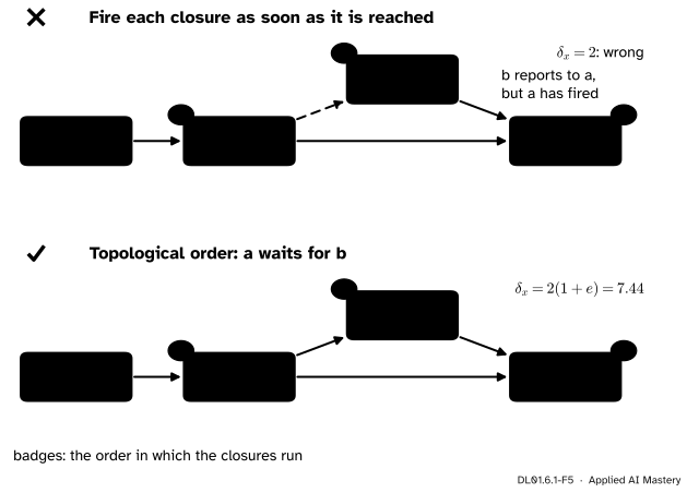
Wrong beside right. The node \(a\) feeds both \(b\) and \(y\). If its closure runs before \(b\) has reported, it passes back only part of its gradient, and \(x\) gets 2 instead of \({2(1 + e)}\).
“Walk back from the output and run each closure when you first reach it.”
A node can be reached before all its children have reported. In the figure the walk reaches \(a\) straight from \(y\), runs its closure with \({\delta_a = 1}\), and only later does \(b\) add \(e\) to \(\delta_a\), which by then goes nowhere. The topological sort exists to stop this: a node’s closure runs only after every node that uses it.
“Changing x.data after the forward pass is harmless.”
The closures read the parents’ arrays when backward runs, not when the forward pass ran. If x.data is changed in place between the two, the gradient is computed at the new values and belongs to no forward pass at all. PyTorch guards against in-place changes of this kind: every tensor carries a version counter, and backward raises an error if a tensor it saved has changed since. This small engine trusts you.
“Calling backward on an array output gives the Jacobian.”
It gives \({\mat{J}\T\vect{1}}\), the gradient of the sum of the outputs. For an elementwise program that happens to list every entry’s derivative, but for a matrix product or a sum it mixes entries. PyTorch refuses to guess: backward() on a tensor with more than one element needs the seed passed in as its gradient argument.
Check yourself
Recall
1. What four things does a Tensor hold?
Show answer
Its data (a NumPy array), its grad (an array of the same shape, zero at first), its parents, and a backward closure that passes its grad back to the parents.
2. What does the backward closure of an elementwise operation \({v = g(u)}\) add to u.grad?
Show answer
\({g'(u) \odot \delta_v}\), the vector-Jacobian product with a diagonal Jacobian, computed with \(n\) multiplications.
3. Why are the closures called in reverse topological order?
Show answer
So that a node’s closure runs only after every node that uses it has added its share to the node’s grad; then the grad it passes back is complete.
4. What does backward compute when the output is an array and the seed is all ones?
Show answer
\({\mat{J}\T\vect{1}}\), the gradient of the sum of the output’s entries.
5. How many nodes does the running program’s graph have when the inputs have a million entries?
Show answer
Seven, as for one entry: one node per input and one per operation. The size of the arrays does not change the size of the graph.
Exercises
1. ★ Add a sigmoid operation, \({\sigma(a) = 1/(1 + e^{-a})}\), to the class, with a backward closure that reuses the forward result. What does it add to a.grad?
Show solution
The derivative is \({\sigma'(a)} = {\sigma(a)\,(1 - \sigma(a))}\), so the closure adds \({\sigma(a)(1 - \sigma(a)) \odot \delta}\), all from the output’s own data:
def sigmoid(self):
    out = Tensor(1 / (1 + np.exp(-self.data)))
    def backward_fn():
        self.grad += out.data * (1 - out.data) * out.grad
    return out.record((self,), backward_fn)
2. ★★ Let \({x = (1, -2, 0.5)}\) and \({y = x^3}\). What is x.grad after one call of y.backward(), and after a second call on the same graph? Why?
Show solution
After one call, \({3x^2 \odot \vect{1}} = {(3,\ 12,\ 0.75)}\). The second call zeroes the grad of \(y\) (a result) and reseeds it, but \(x\) is a leaf and keeps what it holds, so the closure adds \({(3, 12, 0.75)}\) again: \({(6,\ 24,\ 1.5)}\). Leaves accumulate across calls, as in PyTorch, which is why DL01.6.3 needs a zero_grad.
3. ★★★ A program is built only from the elementwise operations of this lesson, on inputs of the same shape. Prove that its Jacobian with respect to each input is diagonal, and conclude that the seed of ones gives every entry’s own derivative.
Show solution
Use induction over the operations in the order they run. Each input is a leaf, and its Jacobian with respect to itself is the identity, which is diagonal; with respect to the other input it is zero, also diagonal. Suppose every tensor computed so far has a diagonal Jacobian with respect to each input. A one-argument operation \({v = g(u)}\) has, by the chain rule, Jacobian \({\operatorname{diag}(g'(u))\,\mat{J}_u}\), a product of diagonal matrices, which is diagonal. A two-argument one, \({a + b}\) or \({a \odot b}\), has \({\mat{J}_a + \mat{J}_b}\) or \({\operatorname{diag}(b)\mat{J}_a} + {\operatorname{diag}(a)\mat{J}_b}\): sums of products of diagonal matrices, again diagonal. So the output’s Jacobian \(\mat{J}\) is diagonal, and entry \(j\) of \({\mat{J}\T\vect{1}}\) is the sum of column \(j\) of \(\mat{J}\), which is its one diagonal entry \({\partial y_j / \partial x_j}\).
Summary card
A tensor engine is the scalar engine with an array at every node.
Same graph, whole arrays.
- A
Tensorholds data, grad, parents and a backward closure. - Backward rule: \({\vect{\delta}_{\vect{u}} \mathrel{+}= \mat{J}\T\vect{\delta}_{\vect{v}}}\).
- Elementwise: \({\vect{\delta}_{\vect{u}} \mathrel{+}= g'(\vect{u}) \odot \vect{\delta}_{\vect{v}}}\).
- Sort topologically, seed ones, call closures in reverse, add.
Sources and next steps
Sources. Each was opened and checked against this lesson on 15 November 2026.
- A. G. Baydin, B. A. Pearlmutter, A. A. Radul and J. M. Siskind, Automatic Differentiation in Machine Learning: a Survey, JMLR 18(153), 2018. Section 3.2 computes the transposed Jacobian-vector product by starting the reverse phase with the seed, and notes the storage cost; section 4.2 explains the terms define-by-run and dynamic computational graph.
- I. Goodfellow, Y. Bengio and A. Courville, Deep Learning, chapter 6. Section 6.5.2 writes the chain rule as a Jacobian-gradient product (equations 6.46 and 6.47, the second for tensors); section 6.5.6 gives every operation its own bprop method (equation 6.54).
- A. Karpathy, micrograd (MIT licence): a scalar reverse-mode engine of about 100 lines over a dynamically built graph. This module follows its closure design but puts arrays at the nodes.
- PyTorch 2.15, Autograd mechanics: the graph’s leaves are the inputs and its roots the outputs, it is recreated at every iteration, a non-differentiable point such as ReLU at 0 takes the subgradient of minimum norm, and a version counter catches in-place changes.
torch.Tensor.backward: a non-scalar output needs agradientargument, and gradients accumulate in the leaves.
Next. DL01.6.2 Matrix products, reductions and broadcasting adds the operations that change shapes, and with them everything a network needs.
This lesson unlocks
DL01.6.2 Matrix products, reductions and broadcasting
Your progress is saved in this browser only. No account, no tracking.