A regression network does not predict a number: it predicts the centre of a bell of possible targets. Minus the log of that bell is the loss. A Gaussian bell gives the mean squared error, a Laplace bell the mean absolute error, and Huber’s loss sits between them.
DL01.4.1L2 Intermediate25 minIn review (what this means)
The maths and code on this page are checked by automated tests on every change, but an independent reader has not signed it off yet. Spot a mistake or a confusing step? Tell us.
State the maximum-likelihood recipe: the network outputs the parameters of a distribution over the target, and the loss is the mean negative log-likelihood.
Derive, line by line, that a Gaussian of fixed variance gives the mean squared error plus a constant, and that a Laplace distribution gives the mean absolute error.
Explain why squared error is pulled hard by an outlier while absolute error and Huber’s loss are not, using the pull each example exerts on the prediction.
Fit a line with each of the three losses by gradient descent and compare the result with scikit-learn’s HuberRegressor.
The question
The linear neuron of DL01.1.1, with the identity activation and the mean squared error, fits the four points of ML01 with the line \({\hat y = 1.4x + 0.5}\). Now a fifth reading arrives: at \({x = 4}\) the sensor reports \({y = 1}\) instead of about 6. One bad number, and the slope of the least-squares line drops from 1.4 to 0.5. Why squared error in the first place, what else could we choose, and how does a network decide how much one strange example should count?
Intuition
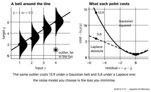
A regression network does not really claim that the target is its output. It claims that the target is probably near its output. Draw that claim as a bell standing sideways on the line: tall at the prediction, falling away on both sides. A target that lands near the peak was expected. A target out in the tail was a surprise.
DL01.4.1-F1
Left: the model as a bell of possible targets around the line, here \({\hat y = 1.4x + 0.5}\). Right: each point’s cost is minus the log of the bell’s height at its target. The outlier costs 13.9 under a Gaussian bell and 5.8 under a Laplace bell.
That surprise is the loss. We score a model by how probable it made the targets we actually saw, and we turn “probable” into a cost by taking minus the logarithm, exactly as the log loss did in ML01.6.2. The only choice left is the shape of the bell. A Gaussian bell has thin tails, so a far-off target is enormously surprising and costs a lot. A Laplace bell has fat tails, so the same target costs much less. Choosing the bell is choosing the loss.
Build it up
Step 1. The Gaussian bell. A Gaussian (or normal) distribution with centre \(\mu\) and width \(\sigma\) gives a target \(y\) the density
You need no probability course to use it: it is a formula for the height of the bell. It is highest at \({y = \mu}\) and falls off with the square of the distance from \(\mu\).
Step 2. One example. Let the network output the centre, \({\mu = \hat y}\), and write the residual as \({r = y - \hat y}\). Take minus the logarithm of the density. The log of a product is a sum of logs, and the log undoes the exponential:
With \({\sigma = 1}\) a point on the line (\({r = 0}\)) costs \({\tfrac12 \ln 2\pi \approx 0.919}\), and the outlier with \({r = -5.1}\) costs \({5.1^2/2 + 0.919 \approx 13.92}\).
Step 3. The Laplace bell. The Laplace distribution with centre \(\mu\) and scale \(b\) has density \({\tfrac{1}{2b} e^{-|y - \mu|/b}}\). Its minus log is
\[
-\ln p(y \mid \hat y, b) = \frac{|r|}{b} + \ln(2b).
\]
With \({b = 1}\) the outlier costs \({5.1 + \ln 2 \approx 5.79}\). The Gaussian cost grows with the square of the residual, the Laplace cost only in proportion to it.
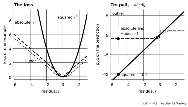
Step 4. What each example does to the line. Gradient descent moves the prediction by minus the slope of the loss. Leave the constants aside and look at three per-example losses: the squared error \(r^2\), the absolute error \(|r|\), and Huber’s loss, which is \({\tfrac12 r^2}\) for \({|r| \le \delta}\) and the straight line \({\delta(|r| - \tfrac12\delta)}\) beyond, here with \({\delta = 1}\).
DL01.4.1-F2
Left: three losses of one example. Right: the pull each exerts on the prediction. Squared error pulls in proportion to the residual, so the outlier pulls with \({-10.2}\); absolute error and Huber’s loss never pull harder than 1.
The pull of the squared error is \({2r}\): the farther the point, the harder it drags the line. The absolute error pulls with \({\pm 1}\) whatever the distance, so a far point has no more say than a near one. Huber’s loss behaves like squared error near the line and like absolute error far from it. That is the whole story of robustness in one picture.
The formal statement
NoteThe maximum-likelihood recipe
Choose a probability distribution \(p(y \mid \vartheta)\) over the target, with parameters \(\vartheta\).
Let the network compute those parameters from the input: \({\vartheta = f(\vect{x}; \theta)}\).
Train by minimising the mean negative log-likelihood of the training set:
The mean of a log is the log of a product, so minimising \(L\) is the same as making the product of the \(n\) probabilities, the likelihood of the data, as large as possible. That is why the recipe is called maximum likelihood. It treats the examples as independent given their inputs, so that their probabilities multiply.
The Gaussian gives the mean squared error. Put Step 2 into the recipe, with \({\hat y_i = f(\vect{x}_i; \theta)}\), residuals \({r_i = y_i - \hat y_i}\), \(\sigma\) fixed and the constant written \({c = \tfrac12\ln(2\pi\sigma^2)}\):
The second line splits the sum in two; the constant is the same for every \(i\), so its mean is itself. The last term does not depend on \(\theta\) and the factor \({1/2\sigma^2}\) is positive, so whatever \(\theta\) makes the MSE smallest also makes \(L\) smallest. The mean squared error is the negative log-likelihood of Gaussian noise, up to a scale and a constant.
The Laplace distribution gives the mean absolute error. The same steps with Step 3 give
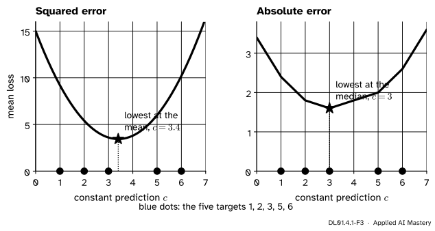
which is zero when \({c = \tfrac1n\sum_i y_i}\): the mean. The derivative of the MAE is \({\tfrac1n}\) times the number of targets below \(c\) minus the number above it, which changes sign where half the targets lie on each side: the median. One far target moves a mean a long way and a median not at all.
DL01.4.1-F3
A constant model for the five targets \({1, 2, 3, 5, 6}\). The squared error is lowest at their mean, 3.4; the absolute error at their median, 3.
Go deeper: letting the network learn the width of the bell
Nothing stops us treating \(\sigma\) as a parameter too. With the MSE fixed, the loss as a function of \(\sigma^2\) is \({\tfrac{1}{2\sigma^2}\mathrm{MSE} + \tfrac12\ln 2\pi + \tfrac12\ln\sigma^2}\). Its derivative with respect to \(\sigma^2\) is \({-\tfrac{\mathrm{MSE}}{2\sigma^4} + \tfrac{1}{2\sigma^2}}\), which is zero at \({\sigma^2 = \mathrm{MSE}}\). For the line \({1.4x + 0.5}\) on the four clean points that is \({\sigma^2 = 0.05}\). A network with a second output for \(\sigma\), kept positive, can even learn a width that changes with the input (Prince, Section 5.3.4).
Worked example
Five points: the four of ML01 and the outlier \({(4, 1)}\).
Least squares. The means are \({\bar x = 14/5 = 2.8}\) and \({\bar y = 17/5 = 3.4}\). The deviations \({x_i - \bar x}\) are \({-1.8, -0.8, 0.2, 1.2, 1.2}\) and the deviations \({y_i - \bar y}\) are \({-1.4, -0.4, 1.6, 2.6, -2.4}\). The slope of ML01.4.2 is
and the intercept is \({\bar y - w\bar x = 3.4 - 1.4 = 2}\). The line is \({\hat y = 0.5x + 2}\): the outlier has cut the slope from 1.4 to 0.5.
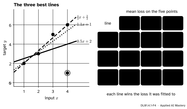
Huber. Try \({\hat y = 1.1x + 1}\). The residuals \({y - \hat y}\) are \({-0.1, -0.2, 0.7, 0.6, -4.4}\). Huber’s pull \(\psi(r)\) is \(r\) itself inside \({[-1, 1]}\) and \({\pm 1}\) outside, so the pulls are \({-0.1, -0.2, 0.7, 0.6, -1}\). The best line makes the total pull zero, and the total pull weighted by \(x\) zero too:
Both hold, and Huber’s mean loss is convex in \({(w, b)}\), so \({1.1x + 1}\) is its best line.
Absolute error. The line through \({(1, 2)}\) and \({(4, 6)}\), \({\hat y = \tfrac43 x + \tfrac23}\), has residuals \({0, -\tfrac13, \tfrac13, 0, -5}\) and a mean absolute error of \({\tfrac{17/3}{5} = \tfrac{17}{15} \approx 1.133}\). The code below confirms with an exact solver that no line does better.
DL01.4.1-F4
The three best lines on the five points, and each line scored by all three losses. Each line is best under its own loss, and only the squared-error line has been dragged by the outlier.
Code
First the three losses and their gradients from scratch, with residuals \({y - \hat y}\) and means over the examples. Each fit is plain gradient descent from \({(0, 0)}\). The absolute error has no slope at \({r = 0}\), so we use its subgradient\(-\mathrm{sign}(r)\) and a step that shrinks like \({1/\sqrt{t}}\); the pitfalls explain why.
import numpy as npx = np.array([1.0, 2.0, 3.0, 4.0, 4.0])y = np.array([2.0, 3.0, 5.0, 6.0, 1.0]) # the four points of ML01 and the outlier (4, 1)def pull(kind, r, delta=1.0):"""Minus the derivative of one example's loss with respect to its prediction."""if kind =="squared":return2* rif kind =="absolute":return np.sign(r)return np.clip(r, -delta, delta) # Huberdef loss(kind, w, b, delta=1.0): r = y - (w * x + b)if kind =="squared":return np.mean(r **2)if kind =="absolute":return np.mean(np.abs(r)) a = np.abs(r)return np.mean(np.where(a <= delta, 0.5* r **2, delta * (a -0.5* delta)))def fit(kind, lr, steps, shrink=False): w = b =0.0for t inrange(steps): g = pull(kind, y - (w * x + b)) eta = lr / np.sqrt(t +1) if shrink else lr w, b = w + eta * np.mean(g * x), b + eta * np.mean(g) # minus a gradient is plus a pullreturn w, bfits = {"squared": fit("squared", 0.05, 2000),"huber": fit("huber", 0.1, 5000),"absolute": fit("absolute", 0.1, 20000, shrink=True)}for kind, (w, b) in fits.items():print(f"{kind:9s} w = {w:.4f} b = {b:.4f} its loss = {loss(kind, w, b):.4f}")
squared   w = 0.5000  b = 2.0000  its loss = 3.1000
huber     w = 1.1000  b = 1.0000  its loss = 0.8700
absolute  w = 1.3324  b = 0.6669  its loss = 1.1337
Gradient descent lands on \({0.5x + 2}\) and \({1.1x + 1}\) to six decimals, and close to \({\tfrac43 x + \tfrac23}\). To be sure the absolute-error line is the best possible, write the MAE as a linear programme, \({\min \sum_i u_i}\) subject to \({u_i \ge \pm(y_i - wx_i - b)}\), and solve it exactly with SciPy:
from scipy.optimize import linprogn =len(x)cost = np.r_[0.0, 0.0, np.ones(n)] # variables: w, b, u_1 ... u_nrows = [np.r_[s * x[i], s, -np.eye(n)[i]] for i inrange(n) for s in (1.0, -1.0)]limits = [s * y[i] for i inrange(n) for s in (1.0, -1.0)]exact = linprog(cost, A_ub=rows, b_ub=limits, bounds=[(None, None)] *2+ [(0, None)] * n)print("exact least-absolute line:", np.round(exact.x[:2], 4), " MAE:", round(exact.fun / n, 4))
scikit-learn’s HuberRegressor uses Huber’s loss with \({\epsilon = 1.35}\), but on residuals divided by a scale \(\sigma\) that it estimates at the same time, and it adds a small L2 penalty \({\alpha\,\lVert w \rVert^2}\) with \({\alpha = 0.0001}\) by default.
from sklearn.linear_model import HuberRegressorhuber = HuberRegressor().fit(x.reshape(-1, 1), y)print(f"HuberRegressor: w = {huber.coef_[0]:.3f}, b = {huber.intercept_:.3f}, scale = {huber.scale_:.3f}")print("flagged as outliers:", huber.outliers_)
HuberRegressor: w = 1.278, b = 0.684, scale = 0.272
flagged as outliers: [False False  True False  True]
Its scale comes out at about 0.27, so its quadratic zone reaches only \({1.35 \times 0.27 \approx 0.37}\) either side of the line. Two points, \({(3, 5)}\) and the outlier, fall outside it and are treated by absolute error, and the line, about \({1.28x + 0.68}\), lands between our Huber line and the absolute-error line. Same idea, a different \(\delta\).
Explore
This module’s interactive, the one-example loss explorer, lives in lesson DL01.4.2, where the same question, how hard does a loss push when the model is badly wrong, is asked of a classifier.
Pitfalls
DL01.4.1-F5
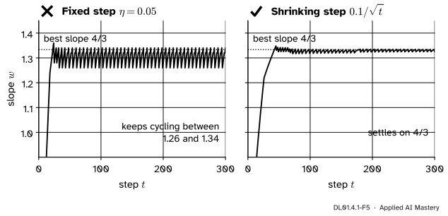
Wrong beside right. With a fixed step, gradient descent on the absolute error never settles: the slope of \({|r|}\) is always 1, so steps do not shrink near the minimum. A shrinking step settles.
“Squared error assumes that my data are Gaussian.”
It assumes that the noise around the prediction is Gaussian, for each input. The inputs, and the targets taken all together, can have any shape at all. The four points of ML01 are not a bell; the residuals from a good line could be.
“A wider bell gives a different best line.”
With \(\sigma\) fixed, the loss is \({\mathrm{MSE}/2\sigma^2}\) plus a constant. Changing \(\sigma\) rescales the loss and so changes the size of each gradient step, like changing the learning rate, but it does not move the minimum. For the same reason the factor \({\tfrac12}\) that some books put in front of the squared error does not matter: it is \({\sigma = 1}\) instead of \({\sigma^2 = \tfrac12}\), and it moves no minimum.
“Absolute error is robust, so it is always the safer choice.”
Two costs come with it. Its gradient has the same size near the minimum as far from it, so plain gradient descent with a fixed step keeps overshooting (figure above); Huber’s loss, quadratic near zero, does not. And when the noise really is Gaussian, the mean uses the data more efficiently than the median. Huber’s loss is the usual compromise.
Check yourself
Recall
1. In the maximum-likelihood recipe, what does the network output, and what is the loss?
Show answer
It outputs the parameters of a distribution over the target, such as the centre of a Gaussian. The loss is the mean over the examples of minus the log of the probability, or density, that distribution gives to the observed target.
2. Which noise distribution turns maximum likelihood into the mean squared error, and what happens to the constant \({\tfrac12\ln(2\pi\sigma^2)}\)?
Show answer
A Gaussian with fixed variance. The constant does not depend on the network’s parameters, so it does not change which parameters are best, and it is dropped.
3. Which distribution gives the mean absolute error?
Show answer
The Laplace distribution, whose minus log density is \({|y - \mu|/b + \ln 2b}\).
4. A constant model is fitted to targets \({1, 2, 3, 5, 6}\). What constant does each loss choose?
Show answer
The mean squared error chooses the mean, 3.4; the mean absolute error chooses the median, 3.
5. How hard does an example with residual \({-5}\) pull the prediction under squared error, absolute error and Huber’s loss with \({\delta = 1}\)?
Show answer
With \({-10}\), \({-1}\) and \({-1}\). Squared error pulls in proportion to the residual; the other two never pull harder than 1 (or \(\delta\)).
Exercises
1.★ Under a Gaussian with \({\sigma = 1}\), what is the cost \({-\ln p}\) of a target 2 units from the prediction? What is it with \({\sigma = 2}\)?
Show solution
The cost is \({r^2/2\sigma^2}\) plus \({\tfrac12\ln(2\pi\sigma^2)}\). With \({\sigma = 1}\): \({4/2 + 0.919 = 2.919}\). With \({\sigma = 2}\): \({4/8} + {\tfrac12\ln(8\pi)} = 0.5 + 1.612 = 2.112\). A wider bell is less surprised by the same miss, but pays a larger constant for being wide.
2.★★ A network with a fixed Laplace scale \(b\) has mean absolute error \(m\) on its training set. Write the loss as a function of \(b\) and find the \(b\) that minimises it.
Show solution
The loss is \({m/b + \ln 2 + \ln b}\). Its derivative with respect to \(b\) is \({-m/b^2 + 1/b}\), which is zero at \({b = m}\). The second derivative there, \({2m/b^3 - 1/b^2 = 1/m^2}\), is positive, so this is a minimum: the best scale is the mean absolute error itself.
3.★★★ Without fitting anything, explain why the Huber line (\({\delta = 1}\)) of the four clean points is \({1.4x + 0.5}\), the least-squares line.
Show solution
The least-squares line has residuals \({y - \hat y}\) of \({0.1, -0.3, 0.3, -0.1}\), all inside \({[-1, 1]}\). There Huber’s loss is \({\tfrac12 r^2}\), half the squared error, so near this line the mean Huber loss is half the MSE and has the same zero gradient. Huber’s mean loss is convex, so a point with zero gradient is its minimum. The line is the same; only an outlier tells the two losses apart.
Summary card
The noise model you choose is the loss you minimise.
DL01.4.1-F1
A bell around the line; surprise is cost.
Recipe.\(L(\theta)\) is the mean of \({-\ln p(y_i \mid f(\vect{x}_i; \theta))}\).
Gaussian, fixed \(\sigma\):\({L = \mathrm{MSE}/2\sigma^2 + \text{const}}\); estimates the mean.
Laplace, fixed \(b\):\({L = \mathrm{MAE}/b + \text{const}}\); estimates the median.
Huber:\({\tfrac12 r^2}\) for \({|r| \le \delta}\), \({\delta(|r| - \tfrac12\delta)}\) beyond; its pull is capped at \(\delta\).
Sources and next steps
Sources. Each was opened and checked against this lesson on 15 November 2026.
Simon J. D. Prince, Understanding Deep Learning, MIT Press, 2023 (free PDF). Section 5.2 gives the recipe in four steps (equation 5.6), Section 5.3 derives the least-squares loss from the normal distribution (equations 5.7 to 5.11), Section 5.3.4 lets the network predict the variance too, and Figure 5.11 lists the Laplace distribution for robust regression.
Ian Goodfellow, Yoshua Bengio and Aaron Courville, Deep Learning, MIT Press, 2016, chapter
Section 6.2.1.1 recovers the mean squared error from a Gaussian model up to a scale and a constant (equation 6.13); Section 6.2.1.2 shows that minimising it predicts the mean (6.14 and 6.15) and the mean absolute error the median (6.16).
Kevin P. Murphy, Probabilistic Machine Learning: An Introduction, MIT Press, 2022 (free online version). Section 11.6.1 uses a Laplace likelihood for robust regression (equation 11.108) and Section 11.6.3 defines Huber’s loss as here (equation 11.117).
scikit-learn 1.9 documentation, HuberRegressor and the User Guide, Section 1.1.14.4. The defaults \({\epsilon = 1.35}\) and \({\alpha = 0.0001}\), the estimated scale scale_, the mask outliers_ and the objective with \(\sigma\).