The two S-shaped activations, their derivatives derived line by line, and the identity that makes tanh a rescaled sigmoid. Then saturation: why a unit whose input lands in a flat tail passes almost no gradient back.
DL01.3.1L2 Intermediate25 minIn review (what this means)
The maths and code on this page are checked by automated tests on every change, but an independent reader has not signed it off yet. Spot a mistake or a confusing step? Tell us.
Derive the derivatives of the sigmoid and of tanh, and show that they are at most 1/4 and 1.
Prove that tanh(z) = 2σ(2z) − 1 and explain what it means for a tanh unit to be centred at zero.
Compute the gradient that a sigmoid or tanh unit passes back, and explain saturation with numbers.
Implement both functions and their derivatives from scratch, with an overflow-safe sigmoid, and check them by central differences and against SciPy and NumPy.
The question
A hidden unit computes \({z = w x + b}\) and passes it through a sigmoid. Training asks it how its weight should change. With \({z = 0.5}\) it answers clearly. With \({z = 6}\) the same unit, fed the same signal from above, answers about 95 times more quietly. Where does the factor 95 come from, and why did it push the field away from S-shaped hidden units?
Intuition
An activation function is the nonlinear step a unit applies to its pre-activation \(z\). Without it, stacked layers collapse into one linear map (DL01.1.4). The two oldest choices are S-shaped: the sigmoid\(\sigma\), which squashes any number into the range 0 to 1, and the hyperbolic tangent\(\tanh\), which squashes it into \(-1\) to \(1\).
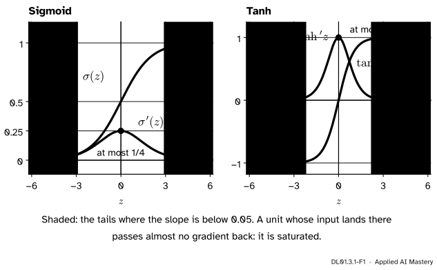
DL01.3.1-F1
Each S-curve (vermillion) with its slope (green). The slope peaks at \(z = 0\): \(1/4\) for the sigmoid, \(1\) for tanh. In the shaded tails it is below 0.05, and the unit is saturated.
Read the green curves. During training, the gradient arriving at a unit’s output is multiplied by the slope of its activation before it travels further back (M05.9.1). Near \(z = 0\) the slope is healthy. Out in the tails the S-curve is flat, the slope is close to zero, and almost nothing gets through. A unit that sits there is saturated: its output hardly changes when its weights do, so gradient descent hardly changes them.
Build it up
Step 1. The sigmoid and its slope. ML01.6.1 met \({\sigma(z) = 1/(1 + e^{-z})}\) as the map from a score to a probability, and ML01.6.3 found its slope, \({\sigma(1 - \sigma)}\). Here the same function sits inside a network, between one layer and the next.
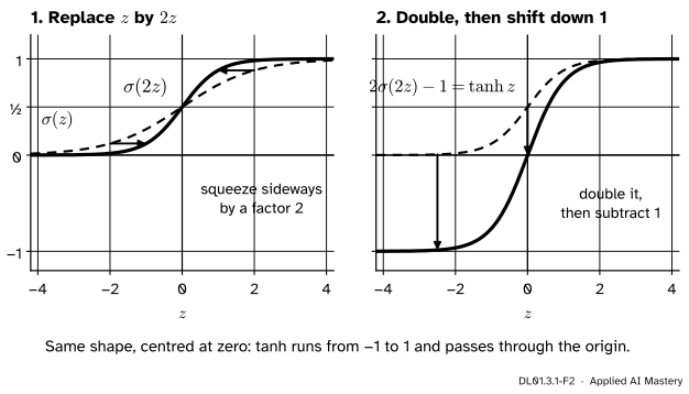
Step 2. Tanh is the same shape. Take the sigmoid, squeeze it sideways by a factor of 2, double its height and shift it down by 1. The result is exactly tanh.
DL01.3.1-F2
Two moves turn the sigmoid into tanh. The shape survives; only the range changes, from 0 to 1 into \(-1\) to \(1\), so tanh is centred at zero.
Step 3. Through one unit. For \({a = \phi(z)}\) with \({z = w x + b}\), the chain rule gives the gradient for the weight in two factors:
The middle factor is the slope of the activation at the unit’s own pre-activation. That is the only place the activation enters the backward pass, so its slope sets how much of the signal the unit lets through.
Their derivatives are \({\sigma'(z) = \sigma(z)\,(1 - \sigma(z))}\), at most \(\tfrac14\), and \({\tanh'(z) = 1 - \tanh^2 z}\), at most 1. Both maxima are at \({z = 0}\). And \({\tanh z = 2\sigma(2z) - 1}\) for every \(z\).
The sigmoid’s derivative. Write \({\sigma = (1 + e^{-z})^{-1}}\) and use the chain rule. The outer power gives \({-(1 + e^{-z})^{-2}}\) and the inner function has derivative \({-e^{-z}}\):
The last step multiplies top and bottom by \(e^{z}\). Differentiating the identity gives a check on both derivatives: \({\tanh'(z) = 4\sigma'(2z)}\), and at \({z = 0}\) that is \({4 \times \tfrac14 = 1}\).
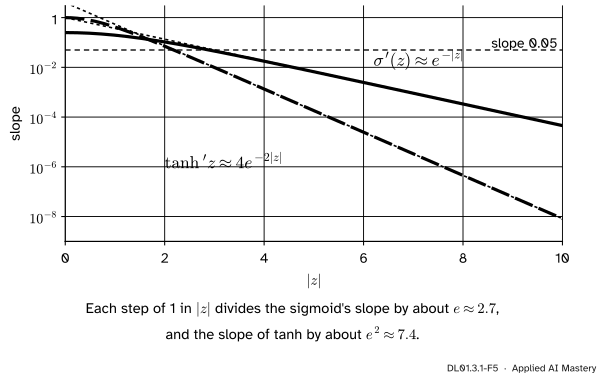
How fast the tails go flat. Write the sigmoid’s slope as \({e^{-z}/(1 + e^{-z})^2}\). For large positive \(z\) the denominator tends to 1, so \({\sigma'(z) \approx e^{-z}}\). Because \({\sigma(-z) = 1 - \sigma(z)}\), the product \({\sigma(1 - \sigma)}\) is the same at \(z\) and \(-z\), so the slope is even and \({\sigma'(z) \approx e^{-\abs{z}}}\) in both tails. Then \({\tanh'(z) = 4\sigma'(2z) \approx 4e^{-2\abs{z}}}\): tanh goes flat twice as fast.
DL01.3.1-F5
On a log scale an exponential is a straight line. The sigmoid’s slope falls by a factor of about \(e\) for each unit of \(\abs{z}\), tanh’s by about \(e^2\).
Solving \({\sigma'(z) = 0.05}\) numerically gives \({\abs{z} \approx 2.887}\), and \({\tanh'(z) = 0.05}\) gives \({\abs{z} \approx 2.178}\). These are the edges of the shaded tails in the first figure.
Worked example
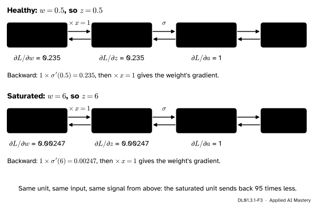
One sigmoid unit, two weights. Take the input \({x = 1}\), no bias, and suppose the layer above sends back \({\partial L/\partial a = 1}\). Compare \({w = 0.5}\) with \({w = 6}\).
DL01.3.1-F3
Forward in black, backward in green. Only the slope \(\sigma'(z)\) differs between the rows, and it is 95 times smaller at \(z = 6\).
Healthy.\({z = 0.5 \times 1 = 0.5}\) and \({a = \sigma(0.5) = 1/(1 + e^{-0.5}) = 0.6225}\). The slope is \({0.6225 \times 0.3775 = 0.2350}\), so \({\partial L/\partial z = 1 \times 0.2350}\) and \({\partial L/\partial w = 0.2350 \times 1 = 0.2350}\).
Saturated.\({z = 6}\) and \({a = 1/(1 + e^{-6}) = 0.99753}\). The slope is \({0.99753 \times 0.00247 = 0.00247}\), and so is \({\partial L/\partial w}\).
The ratio is \({0.2350 / 0.00247 \approx 95}\). Nothing about the loss or the data changed: the second unit simply sits on the flat part of its curve. With tanh in place of the sigmoid the slopes would be \({1 - \tanh^2 0.5 = 0.7864}\) and \({1 - \tanh^2 6 \approx 0.0000246}\), a ratio near 32,000. Tanh passes more back near zero and far less in the tails.
Code
From scratch first. The sigmoid has a trap: \({1/(1 + e^{-z})}\) computes \(e^{800}\) when \({z = -800}\), which overflows, and the rearranged form \({e^{z}/(1 + e^{z})}\) gives infinity over infinity at \({z = 800}\). The safe version picks, for each \(z\), the form whose exponent is never positive.
import numpy as npdef sigmoid(z):"""Overflow-safe: exponentiate only -|z|, which is never positive.""" z = np.asarray(z, dtype=float) e = np.exp(-np.abs(z))return np.where(z >=0, 1/ (1+ e), e / (1+ e))def dsigmoid(z): s = sigmoid(z)return s * (1- s)def tanh(z): e2 = np.exp(-2* np.abs(z)) # tanh is odd, so work with |z| and restore the signreturn np.sign(z) * (1- e2) / (1+ e2)def dtanh(z):return1- tanh(z) **2with np.errstate(all="ignore"): naive_neg =1/ (1+ np.exp(800.0)) # the textbook form at z = -800: e^800 overflows naive_pos = np.exp(800.0) / (1+ np.exp(800.0)) # the other form at z = 800: inf / infprint("naive forms:", naive_neg, naive_pos, " safe:", sigmoid([-800.0, 800.0]))
naive forms: 0.0 nan safe: [0. 1.]
Now check every derivative against central differences, the method of M05.2.4, and check the identity that links the two functions.
The module’s interactive, the activation explorer, lives in lesson DL01.3.4. Choose the sigmoid there and widen the spread of the pre-activations from 2 to 4: the saturated units climb from 4 of 30 to 14, and the mean slope falls from 0.152 to 0.091.
Pitfalls
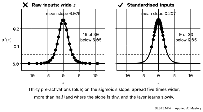
DL01.3.1-F4
Wrong beside right. The same thirty pre-activations, five times wider on the left. More than half fall where the slope is below 0.05; standardised, none do.
“Bigger inputs give the unit more to work with.”
Not with an S-curve. Features measured in large raw units (incomes in pounds, pixel values 0 to 255) make \(\abs{z}\) large from the first step, and the unit starts saturated. Standardise the inputs (ML01.3.3) and start with small weights, so that pre-activations begin near zero, where the slope is largest.
“Sigmoid and tanh are different families, so try both for the same reason.”
They are one shape: \({\tanh z = 2\sigma(2z) - 1}\). What differs is the centre. A sigmoid’s output is always positive, so every input that the next layer receives is positive. The gradient for a weight into a unit is that unit’s \({\partial L/\partial z}\) times the input, so for one example all the weights into a unit get gradients of the same sign, and they can only all rise or all fall together. Tanh outputs have both signs, which is one reason it usually trains better in hidden layers.
“The textbook formula is fine in code.”
\({1/(1 + e^{-z})}\) overflows for large negative \(z\), and \({e^{z}/(1 + e^{z})}\) returns nan for large positive \(z\). Use scipy.special.expit, or the two-branch form above, which never raises a positive number to an exponent.
Check yourself
Recall
1. What is the derivative of the sigmoid in terms of the sigmoid, and what is its largest value?
Show answer
\({\sigma'(z) = \sigma(z)(1 - \sigma(z))}\). It is largest, \(\tfrac14\), at \({z = 0}\), where \({\sigma = \tfrac12}\).
2. What is the derivative of tanh, and its largest value?
Show answer
\({\tanh'(z) = 1 - \tanh^2 z}\), largest at \({z = 0}\), where it equals 1.
3. Write tanh in terms of the sigmoid.
Show answer
\({\tanh z = 2\sigma(2z) - 1}\): squeeze the sigmoid sideways by 2, double it and shift it down by 1.
4. What does it mean for a unit to be saturated, and why does it learn slowly?
Show answer
Its pre-activation lies in a flat tail of its S-curve, where the slope is near zero. The gradient for its weights is multiplied by that slope, so it is tiny.
5. Why does the textbook formula for the sigmoid fail in code, and what is the fix?
Show answer
\({e^{-z}}\) overflows for large negative \(z\) (and the other form gives nan for large positive \(z\)). The fix exponentiates only \({-\abs{z}}\), choosing the form by the sign of \(z\), as scipy.special.expit does.
Exercises
1.★ A tanh unit has \({z = 1}\) and receives \({\partial L/\partial a = 0.5}\) from above. Its input is \({x = 2}\). Find \({\partial L/\partial w}\), using \({\tanh 1 \approx 0.7616}\).
Show solution
The slope is \(1 - 0.7616^2 = 1 - 0.5800 = 0.4200\). Then \(\partial L/\partial w = {0.5 \times 0.4200 \times 2} = 0.4200\).
2.★★ Show that \({\sigma'(-z) = \sigma'(z)}\) and that \({\sigma''(z) = \sigma'(z)\,(1 - 2\sigma(z))}\). Where is the sigmoid’s slope changing fastest?
Show solution
From \({\sigma(-z) = 1 - \sigma(z)}\) (multiply top and bottom of \({1/(1 + e^{z})}\) by \(e^{-z}\)),
Differentiate \({\sigma' = \sigma - \sigma^2}\): \({\sigma'' = \sigma' - 2\sigma\sigma' = \sigma'(1 - 2\sigma)}\). To find where \(\sigma''\) is largest in size, use the same idea once more: \({\sigma''' = \sigma'(1 - 6\sigma + 6\sigma^2)}\), which is zero when \({\sigma = \tfrac12 \pm \tfrac{\sqrt{3}}{6}}\), that is at \({z = \pm\ln(2 + \sqrt{3}) \approx \pm 1.317}\). There the slope changes fastest, rising on the left and falling on the right.
3.★★★ A chain of \(k\) sigmoid units, each \({a_i = \sigma(z_i)}\) with \({z_i = a_{i-1}}\) (weight 1, no bias), starts from \({a_0 = 0}\). Show that the gradient reaching \(z_1\) from the end of the chain is at most \({4^{-k}}\) times \({\partial L/\partial a_k}\), and compute the true factor for \({k = 3}\).
a product of \(k\) slopes each at most \(\tfrac14\), so the factor is at most \({4^{-k}}\). Forward: \({z_1 = 0}\), \({a_1 = 0.5}\); \({z_2 = 0.5}\), \({a_2 = 0.6225}\); \({z_3 = 0.6225}\). The slopes are \({0.25}\), \({0.2350}\) and \({\sigma(0.6225)\,(1 - \sigma(0.6225))}\), which is \({0.6508 \times 0.3492} = 0.2273\). Their product is \({0.25 \times 0.2350 \times 0.2273} \approx 0.0134\), just below the bound \({4^{-3} \approx 0.0156}\). Lesson DL01.3.4 returns to this shrinking.
Summary card
Two S-curves, one shape: steep in the middle, flat in the tails.
Sources. Each was opened and checked against this lesson on 15 November 2026.
Ian Goodfellow, Yoshua Bengio and Aaron Courville, Deep Learning, chapter 6, MIT Press, 2016. Section 6.3.2 states \({\tanh(z) = 2\sigma(2z) - 1}\), describes how sigmoidal units saturate across most of their domain, discourages them as hidden units, and explains why tanh usually does better: it resembles the identity near zero.
Simon J. D. Prince, Understanding Deep Learning, MIT Press, 2023. The notes to chapter 3 contrast the ReLU’s constant slope with sigmoid derivatives that saturate; figure 3.13a draws the sigmoid and tanh.
Stanford CS231n, Neural Networks Part 1, section “Commonly used activation functions”: saturation kills gradients, sigmoid outputs are not centred at zero (so weight gradients share a sign), and tanh is a scaled sigmoid.
SciPy, scipy.special.expit: the logistic sigmoid \({1/(1 + e^{-x})}\), the inverse of logit.