Rosenblatt’s perceptron is a neuron with a step activation that learns only from its mistakes. Work the rule by hand on the AND points, see why each update helps, bound the number of mistakes with Novikoff’s theorem, and watch the rule fail on XOR.
DL01.1.2L2 Intermediate25 minIn review (what this means)
The maths and code on this page are checked by automated tests on every change, but an independent reader has not signed it off yet. Spot a mistake or a confusing step? Tell us.
Apply the perceptron rule by hand to a small data set, tracking every mistake and every update.
Explain why one update moves the boundary towards classifying the mistaken point correctly.
State Novikoff’s convergence theorem with its margin and radius, and check its bound on the AND points.
Show that the rule never settles on data that no line can separate, such as XOR.
Implement the perceptron in NumPy and compare it with scikit-learn’s Perceptron.
The question
In 1958 Frank Rosenblatt described a machine that learned from its mistakes alone. When it classified an example correctly it did nothing; when it got one wrong it nudged its weights. Does such a rule always end with every example classified correctly, and if so, how many mistakes can it make on the way?
From the last lesson
1. Write the two steps a neuron computes.
Show answer
The weighted sum \({z = \vect{w}\T\vect{x} + b}\), then the activation \({\hat{y} = \phi(z)}\).
2. What is \({\pd{L}{z_i}}\) for a sigmoid neuron trained with the mean log loss?
Show answer
\(\frac{1}{n}(p_i - y_i)\), prediction minus target over \(n\).
Intuition
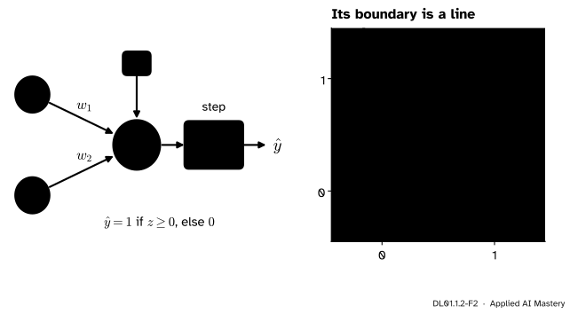
The perceptron is a neuron whose activation is the step: it outputs \({\hat{y} = 1}\) when \({z \geq 0}\) and \({\hat{y} = 0}\) otherwise. Its boundary, the set where \({z = 0}\), is a line in the plane of two inputs, and the perceptron calls everything on one side class 1.
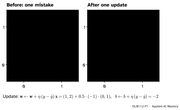
DL01.1.2-F1
One mistake and the update that fixes it. The square at \((0, 1)\) has label \(0\) but sits on the class 1 side. The rule subtracts a little of that point from the weights, and the line moves past it.
The learning rule is as simple as the picture. Go through the examples one at a time. When the perceptron gets one right, change nothing. When it calls a class-0 point class 1, subtract a little of that point from the weights. When it calls a class-1 point class 0, add a little. Each update shifts the line towards the side that classifies the offending point correctly.
Build it up
Step 1. The step activation. The perceptron predicts
With two inputs the boundary \({w_1 x_1 + w_2 x_2 + b = 0}\) is a line. The weight vector \(\vect{w}\) is at right angles to it and points to the side where \({z > 0}\).
DL01.1.2-F2
The perceptron is the neuron of lesson 1 with a step in the activation box. Its answer depends only on which side of the line \({z = 0}\) the input falls.
Step 2. The update rule. For an example \((\vect{x}, y)\) with prediction \(\hat{y}\), and a learning rate \({\eta > 0}\),
The factor \({y - \hat{y}}\) has only three possible values. It is \(0\) when the prediction is right, so nothing changes. It is \(+1\) when a class-1 point was called 0, so \(\eta\vect{x}\) is added. It is \(-1\) when a class-0 point was called 1, so \(\eta\vect{x}\) is subtracted.
Step 3. Why one update helps. Suppose a class-1 point \(\vect{x}\) was called 0, so its \({z < 0}\). After the update its weighted sum is
The added amount is positive, so \(z\) rises towards the right sign. For a class-0 point called 1 the same algebra gives \({z - \eta(\norm{\vect{x}}^2 + 1)}\), a fall. In the figure above, \({\vect{x} = (0, 1)}\) and \({\eta = 0.5}\), so \(z\) falls by \({0.5 \cdot (1 + 1) = 1}\), from \(0.5\) to \(-0.5\). One update may not be enough, and it can break a point that was right before; the rule simply keeps going.
Step 4. Epochs. One pass through all the examples, in a fixed order, is an epoch. Training stops after the first epoch without a mistake, because from then on nothing would change.
The formal statement
NoteDefinition: the perceptron algorithm
Given examples \((\cdata{\vect{x}_i}, \ctruth{y_i})\) with \({y_i \in \{0, 1\}}\) and a learning rate \(\eta > 0\), start from \({\cparam{\vect{w}} = \vect{0}}\), \({\cparam{b} = 0}\). Repeat epochs: for each \(i\) in turn, compute \({\cmodel{\hat{y}_i} = 1}\) if \({\vect{w}\T\vect{x}_i + b \geq 0}\), else \(0\), and apply the update of Step 2. Stop after an epoch with no mistake.
To state the theorem, fold the bias into the weights. Write \({\tilde{\vect{x}} = (\vect{x}, 1)}\) and \({\vect{\theta} = (\vect{w}, b)}\), so that \({z = \vect{\theta}\T\tilde{\vect{x}}}\), and write the label as a sign \({s_i = 2y_i - 1}\), which is \(+1\) or \(-1\). A point is classified correctly with room to spare when \({s_i z_i > 0}\).
NoteTheorem (Novikoff, 1962)
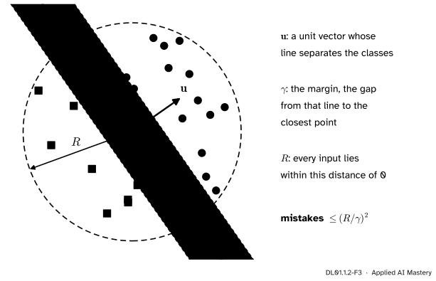
Suppose some unit vector \(\vect{u}\) separates the data with margin\({\gamma > 0}\), meaning \({s_i\,\vect{u}\T\tilde{\vect{x}}_i \geq \gamma}\) for every \(i\), and every input lies within a radius\(R\), meaning \({\norm{\tilde{\vect{x}}_i} \leq R}\). Then the perceptron algorithm, with any \({\eta > 0}\), makes at most \({(R/\gamma)^2}\) mistakes. In particular it stops.
DL01.1.2-F3
The two numbers of the theorem, drawn for inputs whose bias is already folded in (the line passes through the origin). A wide margin and a small radius mean few mistakes.
The bound says nothing about the order of the examples or the size of \(\eta\), and it does not grow with the number of examples. On data that no line separates there is no \(\vect{u}\) with a positive margin, so the theorem is silent, and in fact the rule never stops.
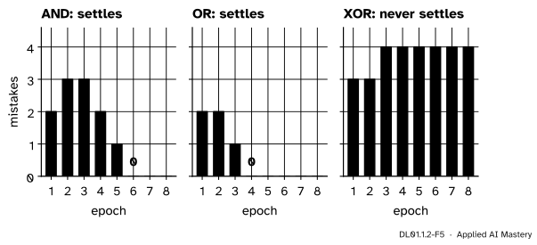
DL01.1.2-F5
Mistakes per epoch from zero weights with \({\eta = 1}\). AND and OR reach an epoch without a mistake; XOR settles into a cycle with four mistakes in every epoch.
On XOR, from epoch 3 on, every epoch ends with the same weights, \({\vect{w} = (-1, 0)}\) and \({b = 0}\), after four mistakes. The rule goes round the same loop for ever.
Go deeper: proof of Novikoff's theorem
Let \(\vect{\theta}_k\) be the weights after \(k\) mistakes, with \({\vect{\theta}_0 = \vect{0}}\). On a mistake at example \(i\) the factor \({y_i - \hat{y}_i}\) equals \(s_i\), so \({\vect{\theta}_k = \vect{\theta}_{k-1} + \eta\,s_i\,\tilde{\vect{x}}_i}\). A mistake also means \({s_i\,\vect{\theta}_{k-1}\T\tilde{\vect{x}}_i \leq 0}\): a class-1 point had \({z < 0}\), or a class-0 point had \({z \geq 0}\).
The weights gain on \(\vect{u}\). Taking the dot product with \(\vect{u}\),
Divide by \({\sqrt{k}\,\eta\gamma}\) to get \({\sqrt{k} \leq R/\gamma}\), that is \({k \leq (R/\gamma)^2}\). The learning rate cancels, which is why the bound does not depend on it.
Worked example
The perceptron on AND, by hand, with \({\eta = 1}\). The points come in the order \((0, 0)\), \((0, 1)\), \((1, 0)\), \((1, 1)\) with labels \(0, 0, 0, 1\). Start from \({\vect{w} = (0, 0)}\), \({b = 0}\).
Epoch 1. At \((0, 0)\), \({z = 0}\), so \({\hat{y} = 1}\): a mistake with \({y - \hat{y} = -1}\). The point is zero, so \(\vect{w}\) stays \((0, 0)\) and \(b\) becomes \(-1\). At \((0, 1)\) and \((1, 0)\), \({z = -1}\): both right. At \((1, 1)\), \({z = -1}\), so \({\hat{y} = 0}\), but the label is \(1\): add the point, giving \({\vect{w} = (1, 1)}\) and \({b = 0}\).
The other epochs go the same way. Every mistake, in order:
Epoch
Mistake at
\(z\)
New \(\vect{w}\), \(b\)
1
\((0, 0)\)
\(0\)
\((0, 0)\), \(-1\)
1
\((1, 1)\)
\(-1\)
\((1, 1)\), \(0\)
2
\((0, 0)\)
\(0\)
\((1, 1)\), \(-1\)
2
\((0, 1)\)
\(0\)
\((1, 0)\), \(-2\)
2
\((1, 1)\)
\(-1\)
\((2, 1)\), \(-1\)
3
\((0, 1)\)
\(0\)
\((2, 0)\), \(-2\)
3
\((1, 0)\)
\(0\)
\((1, 0)\), \(-3\)
3
\((1, 1)\)
\(-2\)
\((2, 1)\), \(-2\)
4
\((1, 0)\)
\(0\)
\((1, 1)\), \(-3\)
4
\((1, 1)\)
\(-1\)
\((2, 2)\), \(-2\)
5
\((0, 1)\)
\(0\)
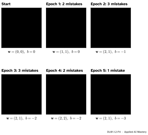
\((2, 1)\), \(-3\)
In epoch 6 the four weighted sums are \(-3\), \(-2\), \(-1\) and \(0\), all on the correct side, so the algorithm stops with \({\vect{w} = (2, 1)}\), \({b = -3}\) after 11 mistakes.
DL01.1.2-F4
The trace, epoch by epoch. Each panel shows the line at the end of the epoch, with the points that caused a mistake during it ringed. After epoch 5 every point is on its side.
The bound. Fold in the bias: the inputs become \({(0, 0, 1)}\), \({(0, 1, 1)}\), \({(1, 0, 1)}\) and \({(1, 1, 1)}\), so \({R = \sqrt{3}}\), the length of the last. Take \({\vect{u} = (2, 2, -3)/\sqrt{17}}\), the line \({x_1 + x_2 = 1.5}\). The signed values \({s_i\,\vect{u}\T\tilde{\vect{x}}_i}\) are \(3/\sqrt{17}\) for \((0, 0)\) and \(1/\sqrt{17}\) for the other three, so \({\gamma = 1/\sqrt{17} \approx 0.243}\) and
The perceptron made 11 mistakes, well inside the bound of 51. (No other \(\vect{u}\) has a wider margin on these points; the code below checks it.)
Look at the \(z\) column once more: seven of the eleven mistakes happen at \({z = 0}\), a point lying exactly on the line. With integer data and \({\eta = 1}\) that is common, and it is why the rule for a tie, “\({z \geq 0}\) means class 1”, must be stated.
Code
The perceptron from scratch. It returns the weights and the number of mistakes in each epoch.
import numpy as npdef perceptron(X, y, lr=1.0, epochs=20, ties_are_mistakes=False):"""Rosenblatt's rule in a fixed order, from zero weights. Stops after an epoch with no mistake.""" w, b = np.zeros(X.shape[1]), 0.0 counts = []for _ inrange(epochs): mistakes =0for xi, yi inzip(X, y): z = xi @ w + b yhat =1.0if z >=0else0.0 sign =2* yi -1# +1 for class 1, -1 for class 0if yhat != yi or (ties_are_mistakes and z ==0): w = w + lr * sign * xi # equals lr * (y - yhat) * x on a mistake b = b + lr * sign mistakes +=1 counts.append(mistakes)if mistakes ==0:breakreturn w, b, countsX = np.array([[0.0, 0.0], [0.0, 1.0], [1.0, 0.0], [1.0, 1.0]])gates = {"AND": np.array([0.0, 0.0, 0.0, 1.0]), "OR": np.array([0.0, 1.0, 1.0, 1.0]),"XOR": np.array([0.0, 1.0, 1.0, 0.0])}for name, y in gates.items(): w, b, counts = perceptron(X, y, epochs=10)print(f"{name}: w = {w}, b = {b:4.1f}, mistakes per epoch {counts}")
AND: w = [2. 1.], b = -3.0, mistakes per epoch [2, 3, 3, 2, 1, 0]
OR: w = [1. 1.], b = -1.0, mistakes per epoch [2, 2, 1, 0]
XOR: w = [-1.  0.], b =  0.0, mistakes per epoch [3, 3, 4, 4, 4, 4, 4, 4, 4, 4]
The theorem’s two numbers for AND, and a check that no direction beats the margin of \({\vect{u} = (2, 2, -3)/\sqrt{17}}\): a search over a fine grid of unit vectors finds nothing wider.
Xt = np.hstack([X, np.ones((4, 1))]) # fold the bias in: (x1, x2, 1)s =2* gates["AND"] -1R = np.linalg.norm(Xt, axis=1).max()u = np.array([2.0, 2.0, -3.0]) / np.sqrt(17)gamma = (s * (Xt @ u)).min()print(f"R = {R:.4f}, gamma = {gamma:.4f}, bound = {(R / gamma) **2:.1f}")angles = np.linspace(0, np.pi, 721) # unit vectors on a grid over the spherea, c = np.meshgrid(angles, 2* angles)U = np.stack([np.sin(a) * np.cos(c), np.sin(a) * np.sin(c), np.cos(a)], axis=-1).reshape(-1, 3)best = (s * (U @ Xt.T)).min(axis=1).max()print(f"widest margin on the grid: {best:.4f}")
R = 1.7321, gamma = 0.2425, bound = 51.0
widest margin on the grid: 0.2406
Now scikit-learn. Its Perceptron is a stochastic-gradient classifier with a constant step of \({\eta = 1}\) and no penalty. shuffle=False keeps our order and tol=None makes it run every epoch.
from sklearn.linear_model import Perceptronclf = Perceptron(shuffle=False, tol=None, max_iter=20).fit(X, gates["AND"])print("scikit-learn:", clf.coef_[0], clf.intercept_[0], " accuracy", clf.score(X, gates["AND"]))w_tie, b_tie, c_tie = perceptron(X, gates["AND"], ties_are_mistakes=True)print("ours, a tie counted as a mistake:", w_tie, b_tie, c_tie)
scikit-learn: [3. 2.] -4.0  accuracy 1.0
ours, a tie counted as a mistake: [3. 2.] -4.0 [2, 3, 3, 2, 2, 3, 2, 1, 0]
scikit-learn separates AND too, but with \({\vect{w} = (3, 2)}\) and \({b = -4}\), not our \({(2, 1)}\) and \(-3\). The difference is the tie. scikit-learn’s perceptron loss is a hinge loss with threshold 0, whose gradient is non-zero whenever \({s\,z \leq 0}\), so it updates on a point exactly on the line whichever its class. With that one change our function gives its weights exactly, and its final line has no point on it.
Explore
DL01.1-X1
Neuron playground
A neuron with two inputs over the four corner points. Move \(w_1\), \(w_2\) and \(b\), pick the activation, and press Perceptron step to apply the rule to the next mistake.
Three things to try. Press Perceptron step once from the opening state: it is the update of the anchor figure. Press Start from zero, set \(\eta\) to \(1\) and press Train: the read-out gives the mistakes per epoch of the worked example, 2, 3, 3, 2, 1, 0. Then choose XOR and try any sliders you like; the count never reaches 4 of 4.
Pitfalls
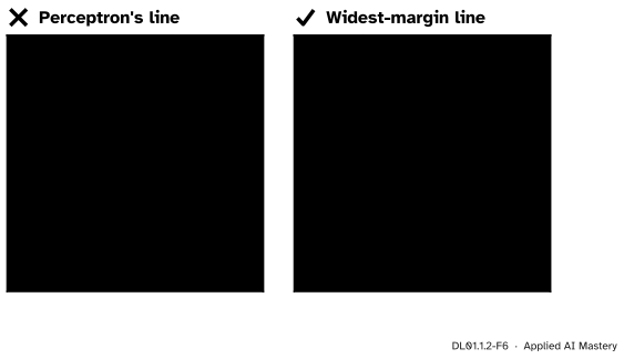
DL01.1.2-F6
Wrong beside right. Left: the perceptron stops at the first line that works, here one that touches \((1, 1)\). Right: the line with the widest gap to the nearest points.
“When the perceptron stops, it has found the best line.”
It has found a line, the first one that makes no mistake, and that line may graze a point. Its final AND line passes through \((1, 1)\) itself, so the point \((1, 0.95)\), which looks like \((1, 1)\), is called 0. The line \({x_1 + x_2 = 1.5}\) keeps a gap of \({0.5/\sqrt{2} \approx 0.35}\) on both sides. Choosing the widest gap is the idea of the support vector machine in ML02.7.
“If it has not settled yet, run it for longer.”
On data that no line separates, such as XOR, the rule never settles: it cycles for ever, and the weights it holds when you stop depend only on when you stopped. Before training longer, ask whether a separating line can exist at all. Lesson 4 proves that for XOR it cannot.
“A smaller learning rate makes the perceptron more careful.”
From zero weights, every update adds \(\pm\eta\tilde{\vect{x}}\), so after any number of steps the weights are exactly \(\eta\) times the weights for \({\eta = 1}\). Scaling \(z\) by a positive number never changes its sign, so every prediction, every mistake and the final line are the same. Only the size of the numbers changes.
Check yourself
Recall
1. Write the perceptron’s update rule for \(\vect{w}\) and \(b\).
Show answer
\({\vect{w} \leftarrow \vect{w} + \eta(y - \hat{y})\vect{x}}\) and \({b \leftarrow b + \eta(y - \hat{y})}\).
2. What does the rule do when the prediction is right?
Show answer
Nothing: \({y - \hat{y} = 0}\), so the weights and the bias do not change.
3. After an update on a class-1 point that was called 0, by how much does that point’s \(z\) change?
Show answer
It rises by \({\eta(\norm{\vect{x}}^2 + 1)}\).
4. State the bound of Novikoff’s theorem and say what \(R\) and \(\gamma\) are.
Show answer
At most \({(R/\gamma)^2}\) mistakes, where \(R\) bounds the length of every input (with the bias folded in as a \(1\)) and \(\gamma\) is the margin of some unit vector that separates the data.
5. What happens when the perceptron is run on XOR?
Show answer
It never settles. From zero weights with \({\eta = 1}\) it makes four mistakes in every epoch from the third on, ending each epoch at \({\vect{w} = (-1, 0)}\), \({b = 0}\).
Exercises
1.★ Run the perceptron by hand on the OR points (labels \(0, 1, 1, 1\) in the order \((0, 0)\), \((0, 1)\), \((1, 0)\), \((1, 1)\)) from zero weights with \({\eta = 1}\). List every mistake.
Show solution
Epoch 1: at \((0, 0)\), \({z = 0}\) gives 1, a mistake: \({b = -1}\). At \((0, 1)\), \({z = -1}\) gives 0, a mistake: \({\vect{w} = (0, 1)}\), \({b = 0}\). Then \((1, 0)\) has \({z = 0}\) and \((1, 1)\) has \({z = 1}\): both right. Epoch 2: \((0, 0)\) has \({z = 0}\), a mistake: \({b = -1}\). \((0, 1)\) has \({z = 0}\): right. \((1, 0)\) has \({z = -1}\), a mistake: \({\vect{w} = (1, 1)}\), \({b = 0}\). \((1, 1)\): right. Epoch 3: \((0, 0)\) has \({z = 0}\), a mistake: \({b = -1}\). The rest are right. Epoch 4: the sums are \(-1\), \(0\), \(0\) and \(1\), all right. Five mistakes; the final line is \({x_1 + x_2 = 1}\).
2.★★ Prove that, starting from zero weights, running the perceptron with learning rate \(\eta\) gives exactly \(\eta\) times the weights obtained with \({\eta = 1}\) after every step, and hence the same predictions.
Show solution
By induction on the number of examples seen. Both runs start at \(\vect{0}\), and \({\vect{0} = \eta \cdot \vect{0}}\). Suppose that before some example the run with rate \(\eta\) holds \({\eta\vect{\theta}}\) while the other holds \(\vect{\theta}\). Their weighted sums are \({\eta z}\) and \(z\), which have the same sign because \({\eta > 0}\), so the two runs make the same prediction. If it is wrong, the first adds \({\eta s\tilde{\vect{x}}}\) and the second adds \({s\tilde{\vect{x}}}\), giving \({\eta(\vect{\theta} + s\tilde{\vect{x}})}\) and \({\vect{\theta} + s\tilde{\vect{x}}}\). The relation holds again.
3.★★★ For OR, show that \({\vect{u} = (2, 2, -1)/3}\) separates the folded-in inputs with margin \({\gamma = 1/3}\), and give the bound of Novikoff’s theorem. Compare it with exercise 1.
Show solution
\(\vect{u}\) has length \({\sqrt{4 + 4 + 1}/3 = 1}\). For \((0, 0, 1)\), label 0, the sign is \(-1\) and \({s\,\vect{u}\T\tilde{\vect{x}} = -(-1/3) = 1/3}\). For \((0, 1, 1)\) and \((1, 0, 1)\) it is \({(2 - 1)/3 = 1/3}\), and for \((1, 1, 1)\) it is \({(4 - 1)/3 = 1}\). The smallest is \(1/3\), so \({\gamma = 1/3}\). With \({R = \sqrt{3}}\) the bound is \({3 \cdot 9 = 27}\) mistakes. The perceptron made 5, again well inside.
Summary card
Change the weights only when wrong, and only by the point you got wrong.
DL01.1.2-F1
One mistake, one nudge.
Prediction.\({\hat{y} = 1}\) if \({\vect{w}\T\vect{x} + b \geq 0}\), else \(0\).
Novikoff. Separable with margin \(\gamma\) and radius \(R\): at most \({(R/\gamma)^2}\) mistakes.
AND. 11 mistakes in 5 epochs, final \({\vect{w} = (2, 1)}\), \({b = -3}\); bound 51.
XOR. Never settles.
Sources and next steps
Sources. Each was opened and checked against this lesson on 15 November 2026.
Simon J. D. Prince, Understanding Deep Learning (MIT Press, 2023), notes to Chapter 3, “History of neural networks”: Rosenblatt (1958) developed the perceptron, which linearly combined inputs and thresholded them, and provided an algorithm to learn the weights from data.
David Chiang, Theory of Neural Networks, Chapter 2: Perceptrons, University of Notre Dame CSE 60963, version of 4 September 2024. Theorem 2.7 (Novikoff, 1962): data linearly separable with margin \(\gamma\), with \({R = \max_i \norm{\vect{x}_i}}\), is separated after at most \(R^2/\gamma^2\) mistakes; the bias is folded in as a feature that is always 1.
Kilian Weinberger, Cornell CS4780 lecture notes: The Perceptron. Absorbs the bias by adding a constant dimension, updates \({\vect{w} \leftarrow \vect{w} + y\vect{x}}\) on a mistake (labels \(\pm 1\)), proves that with inputs scaled into the unit sphere the algorithm makes at most \(1/\gamma^2\) mistakes (the case \({R = 1}\) of the theorem here) by the same two steps, and notes that on data that is not linearly separable it loops forever.
Ian Goodfellow, Yoshua Bengio and Aaron Courville, Deep Learning, Section 1.2.1, on the perceptron (Rosenblatt, 1958) as the first model able to learn the weights that define categories from examples.
scikit-learn 1.9.1 documentation, Perceptron: equivalent to SGDClassifier(loss="perceptron", eta0=1, learning_rate="constant", penalty=None), with defaults shuffle=True and tol=1e-3. The tie rule is in the source, _sgd_fast.pyx.tp: the class Hinge with threshold 0 gives “the loss used by the Perceptron”, and its gradient is non-zero when the product of label and score is at most the threshold.
Next.DL01.1.3 A layer of neurons puts several neurons side by side on the same input and writes them as one matrix.