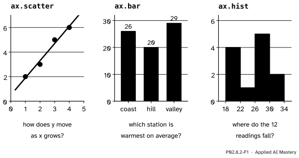
Three more calls on the same Axes, each for one kind of question: ax.scatter for two numeric columns, ax.bar for one number per category, ax.hist for the spread of one column. Count a histogram by hand, check it against NumPy, and see how the choice of bins changes the picture.
P02.8.2L1 Core25 minIn review (what this means)
The maths and code on this page are checked by automated tests on every change, but an independent reader has not signed it off yet. Spot a mistake or a confusing step? Tell us.
Choose between a scatter plot, a bar chart and a histogram from the question being asked.
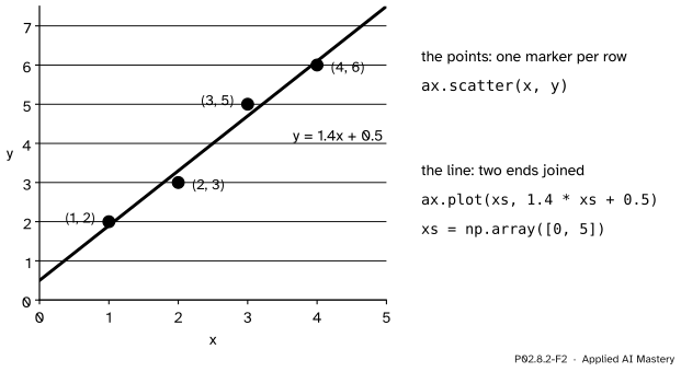
Draw the ML01 points with ax.scatter and the line y = 1.4x + 0.5 through them with ax.plot.
Draw one number per category with ax.bar, and explain why bars must start at zero.
Count a histogram by hand with half-open bins and check it against np.histogram and ax.hist.
Show that moving the bin edges changes the shape a histogram suggests.
The question
Three questions about the same weather data: does one number move with another, which station is warmest, and where do the twelve readings fall? Each wants a different chart. Which one, and how does a histogram decide how tall each bar should be?
From the last lesson
1. With y limits 24 to 34 and a box 300 pixels high, how far down from the top does 28 °C land?
Show answer
\({34 - 28} = 6\) degrees below the top, at 30 pixels a degree: 180 pixels.
2. What is the difference between an Axes and an Axis?
Show answer
An Axes is a plotting area with its own limits; an Axis is one of its two number lines, with ticks and tick labels.
Intuition
A line plot joins points in order, so it suits values that follow one another, such as days or training epochs. Three other shapes of question come up all the time.
Two numbers per row. Does \(y\) grow with \(x\)? Draw each row as a dot at \({(x, y)}\): a scatter plot. No line joins the dots, because the rows have no order.
One number per category. Which station is warmest on average? Draw a bar for each category whose height is the number: a bar chart.
The spread of one column. Where do the readings fall? Cut the number line into intervals called bins, count the readings in each, and draw a bar per bin: a histogram.
P02.8.2-F1
Three calls for three kinds of question. Each draws on an Axes exactly as ax.plot did, through the same scale.
The scatter and the bar chart only place marks. The histogram first computes: it turns twelve readings into four counts, and the counts depend on where the bins start. That computing step is the part to understand before trusting one.
Build it up
Step 1. Scatter. The ML01 regression points are \(x = 1, 2, 3, 4\) and \(y = 2, 3, 5, 6\). ax.scatter(x, y) puts one marker at each pair, through the scale of P02.8.1.
Step 2. A model’s line on top. The line \(y = 1.4x + 0.5\) of ML01 is straight, so two ends are enough: at \(x = 0\) it is \(0.5\) and at \(x = 5\) it is \(7.5\). ax.plot([0, 5], [0.5, 7.5]) joins them. Data as dots, the model as a line: that is a common first check of a fitted model.
P02.8.2-F2
Two calls on one Axes. The scatter shows the data; the line shows the model’s prediction for every \(x\), so the gaps between dots and line are its errors.
Step 3. Bars. The station means of temps are 26, 20 and 29 (P02.2.2). ax.bar(stations, means) takes the category names as the \(x\) values and draws a bar from 0 up to each mean.
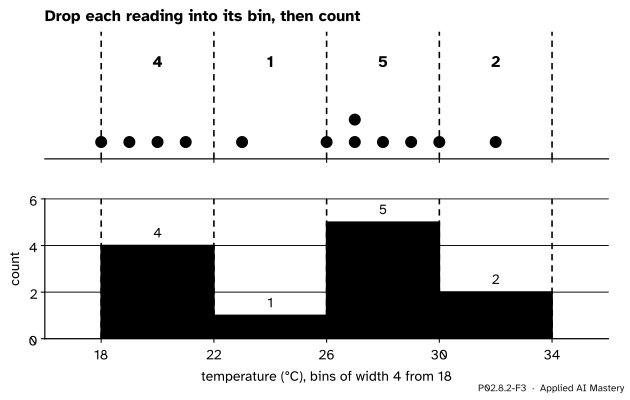
Step 4. Bins. For a histogram of the twelve readings, choose bins of width 4 starting at 18: the edges 18, 22, 26, 30 and 34 make four bins.
Step 5. Count. Go through the readings and add one to the bin each falls in. The counts become the bar heights. ax.hist(values, bins=edges) does the counting and the drawing in one call.
The formal statement
NoteDefinition: histogram counts
Given edges \(e_0 < e_1 < \dots < e_k\), there are \(k\) bins. Bin \(j\) holds the values \(v\) with \(e_{j-1} \le v < e_j\), except the last bin, which also holds \(v = e_k\). The count of a bin is the number of values it holds, and a histogram draws a bar of that height over each bin.
So every bin but the last is half-open: it includes its left edge and leaves out its right one. NumPy’s documentation states this rule for np.histogram, with the edges \([1, 2, 3, 4]\) as its example, and ax.hist calls np.histogram to do its counting.
Why the rule is built that way. A reading that sits exactly on an inner edge, such as 22, could belong to either neighbouring bin. If both took it, it would be counted twice; if neither took it, it would be lost. Leaving out the right edge gives it to exactly one bin, the one on its right. The last bin has no bin to its right, so it keeps its right edge, and a value equal to the largest edge is still counted. Each value inside the range is therefore counted exactly once, and the counts add up to the number of values. Values outside the range from \(e_0\) to \(e_k\) are not counted at all.
P02.8.2-F4
The half-open rule with edges from 16. A reading on an inner edge goes to the bin on its right; the largest edge belongs to the last bin.
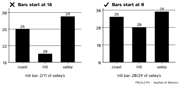
The bar chart has a rule of its own. A bar’s length is what the eye compares: a bar twice as long reads as twice as much. That is only true if every bar starts at zero, so ax.bar starts its axis at zero unless you tell it otherwise. A line or a scatter has no such rule: there the eye reads positions and slopes, not lengths.
Worked example
Count the twelve readings into the bins 18 to 22, 22 to 26, 26 to 30 and 30 to 34.
The readings, day by day and station by station, are 21, 19, 26, 27, 23, 28, 27, 18, 30, 29, 20 and 32. Sorted they are 18, 19, 20, 21, 23, 26, 27, 27, 28, 29, 30, 32.
P02.8.2-F3
The histogram by hand. Each reading drops into one bin; the counts become the bar heights.
\([18, 22)\): 18, 19, 20 and 21. Count 4.
\([22, 26)\): 23 only. Count 1. (26 is not here: the bin leaves out its right edge.)
\([26, 30)\): 26, 27, 27, 28 and 29. Count 5.
\([30, 34]\): 30 and 32. Count 2. (30 sits on an edge and goes to the bin on its right.)
Check: \(4 + 1 + 5 + 2 = 12\), every reading counted once. The picture has a dip at 22 to 26 and a peak at 26 to 30.
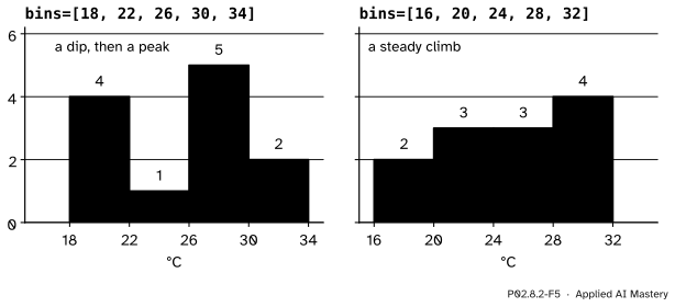
Now start the bins at 16 instead, with edges 16, 20, 24, 28 and 32. The counts become 2 (18 and 19), 3 (20, 21, 23), 3 (26, 27, 27) and 4 (28, 29, 30, 32). Here 20 and 28 sit on inner edges and go right, and 32 is the last edge, kept by the last bin. Same data, but now a steady climb with no dip.
Code
The data and the scatter with the model’s line. The cell closes the figure instead of showing it.
A bar for each station mean. The bar chart’s y axis starts at zero without being asked.
means = temps.mean(axis=0)fig, ax = plt.subplots(figsize=(4, 3))bars = ax.bar(stations, means)print([float(bar.get_height()) for bar in bars])print("y axis starts at", ax.get_ylim()[0])plt.close(fig)
[26.0, 20.0, 29.0]
y axis starts at 0.0
The histogram from scratch, with the half-open rule written out.
def count_bins(values, edges):"""Count values into the bins between consecutive edges; only the last bin keeps its right edge.""" counts = [0] * (len(edges) -1)for v in values:for j inrange(len(counts)): last = j ==len(counts) -1if edges[j] <= v < edges[j +1] or (last and v == edges[-1]): counts[j] +=1breakreturn countsvalues = temps.ravel().tolist()print(values)print(count_bins(values, [18, 22, 26, 30, 34]))print(count_bins(values, [16, 20, 24, 28, 32]))
The two sets of bins from the code, drawn side by side. Twelve readings are too few for any bin choice to be trusted on its own.
Explore
This module’s interactive, Figure anatomy, is in lesson P02.8.1. Moving its y limits shows on a line plot what the pitfall below shows on bars: the limits decide how big a difference looks. Choosing bins with care, and a tool for trying many widths, is the subject of S01.4.1.
Pitfalls
P02.8.2-F6
Wrong beside right. Cut at 18, the hill’s bar is less than a fifth of the valley’s; from zero it is more than two thirds, which is the truth.
“I can zoom a bar chart in on the interesting part.”
A bar is read by its length. Start the axis at 18 and the hill’s bar is \({20 - 18} = 2\) units long beside the valley’s \({29 - 18} = 11\): it looks less than a fifth as warm, when its mean is \({20/29}\), about 0.69, of the valley’s. If the differences are what matter, plot the differences, or use dots on a line, which carry no length. ax.bar starts at zero for this reason; ax.set_ylim(18, 31) undoes it.
“A histogram shows the shape of the data.”
It shows the shape of the data and of the bins. Starting the same bins of width 4 at 18 or at 16 gave a dip and a peak, or a steady climb. With few values, try several bin choices before describing a shape; with many values the choice matters less, but it never vanishes.
“A value on an edge goes in the bin to its left.”
Only the largest edge does. Every other bin leaves out its right edge, so 22 belongs to the bin from 22 to 26, not the one from 18 to 22. A value outside the outer edges is not counted at all, so check that the counts add up to the number of values: 12 here.
Check yourself
Recall
1. Which chart suits each question: does \(y\) grow with \(x\); which category is largest; where do the values of one column fall?
Show answer
A scatter plot, a bar chart and a histogram.
2. Why is the line \(y = 1.4x + 0.5\) drawn with only two points?
Show answer
A straight line is fixed by two points; ax.plot joins them, here at \(x = 0\) and \(x = 5\), giving \(y = 0.5\) and \(7.5\).
3. With the edges 18, 22, 26, 30, 34, which bin holds the reading 26?
Show answer
The bin from 26 to 30: bins include their left edge and leave out their right one.
4. What are the counts for bins of width 4 from 18, and from 16?
Show answer
From 18: 4, 1, 5, 2. From 16: 2, 3, 3, 4.
5. Why must a bar chart’s axis start at zero?
Show answer
Because the eye compares bar lengths; cutting the axis makes the lengths lie about the ratios between the values.
Exercises
1.★ Count the hill column, 19, 23, 18 and 20, into bins of width 2 from 18: edges 18, 20, 22, 24. Then check with np.histogram.
Show solution
\([18, 20)\) holds 18 and 19: count 2. \([20, 22)\) holds 20: count 1. \([22, 24]\) holds 23: count 1. The counts are 2, 1, 1, adding up to 4, and np.histogram([19, 23, 18, 20], bins=[18, 20, 22, 24]) returns the same.
2.★★ax.hist(values, bins=4) asks for four bins of equal width without naming the edges. NumPy then spreads the bins from the smallest value, 18, to the largest, 32. Find the edges and the counts by hand.
Show solution
The range is \({32 - 18} = 14\), so each bin is \({14 / 4} = 3.5\) wide, with edges 18, 21.5, 25, 28.5 and 32. Counting: 18, 19, 20, 21 make 4; 23 makes 1; 26, 27, 27, 28 make 4; and 29, 30, 32 make 3, since 32 is the last edge. The counts are 4, 1, 4, 3: a third picture of the same twelve readings.
3.★★★ Model residuals are \(y - \hat y\). For the ML01 points and the line \(\hat y = 1.4x + 0.5\), compute them, and draw by hand the histogram with edges \(-0.5, 0, 0.5\). Why is a histogram of residuals a common check after fitting a model?
Show solution
The predictions are 1.9, 3.3, 4.7 and 6.1, so the residuals are \({2 - 1.9} = 0.1\), \({3 - 3.3} = -0.3\), \({5 - 4.7} = 0.3\) and \({6 - 6.1} = -0.1\). Two are in \([-0.5, 0)\) and two in \([0, 0.5]\): counts 2 and 2. A histogram of residuals shows whether the errors are centred on zero and how spread out they are; a lopsided one, or a long tail, says the model misses in a pattern.
Summary card
Pick the chart from the question; a histogram counts before it draws.
P02.8.2-F1
Scatter, bar, histogram.
ax.scatter(x, y): two numbers per row, no line between rows.
ax.bar(categories, heights): one number per category; bars start at zero.
ax.hist(values, bins=edges): counts per bin, bins include their left edge and leave out their right one, except the last.
The bins are a choice: the same data from 18 give 4, 1, 5, 2 and from 16 give 2, 3, 3, 4.
Sources and next steps
Sources. Each was opened and checked against this lesson on 15 November 2026.
NumPy developers, numpy.histogram, NumPy 2.5 manual. The Notes state that all but the last bin are half-open, with the edges \([1, 2, 3, 4]\) as the example: the last bin, \([3, 4]\), includes 4.
Matplotlib developers, matplotlib.axes.Axes.hist, Matplotlib 3.11.2: the method uses numpy.histogram to bin the data and count the values in each bin, returns the tuple (counts, edges, patches), and with an integer bins makes that many equal-width bins between the smallest and the largest value.
Matplotlib developers, Quick start guide, Matplotlib 3.11.2: plotting functions expect NumPy arrays or anything numpy.asarray accepts (Types of inputs to plotting functions), and strings such as station names give categorical plotting (Plotting dates and strings).
Next.P02.8.3 Several panels, one style puts three charts side by side on one shared scale. Reading distributions properly is S01.4, and choosing a chart for a question is P04.3.
![A number line from 16 to 32 with orange dashed lines at the edges 16, 20, 24, 28 and 32, and the bins named [16, 20), [20, 24), [24, 28) and [28, 32] in orange. The twelve readings are dots on the line, stacked where a value repeats. Three dots sit exactly on an edge and are vermillion: 20 and 28, each with a green arrow pointing right and the words goes right, and 32, with a green arrow pointing left and the words stays in. Below: bins from 16 to 32 give the counts 2, 3, 3, 4; a value above 32 would be left out.](figures/P02.8.2-F4.svg)