One whole-array expression replaces a Python loop. Compute predictions, residuals and the mean squared error of a line on four points, first with a loop and then in one line each, and see why NumPy’s version is so much faster.
P02.2.1L1 Core25 minIn review (what this means)
The maths and code on this page are checked by automated tests on every change, but an independent reader has not signed it off yet. Spot a mistake or a confusing step? Tell us.
Rewrite a Python loop over the entries of an array as one whole-array expression.
Predict the result of arithmetic, comparisons and universal functions such as np.sqrt and np.abs applied to an array.
Compute the predictions, residuals and mean squared error of a line on four points with a loop and with NumPy, and check that they agree.
Explain why the vectorised version is faster, and time both versions with time.perf_counter.
Tell the element-wise product * from the matrix product @.
The question
A line \(\hat y = 1.4x + 0.5\) has to be scored on a million points. In plain Python that is a loop of a million turns for the predictions, another for the errors, and a third for their squares. NumPy does the same work in one line per step, and finishes many times sooner. Where did the loops go, and why does moving them make such a difference?
Intuition
In P02.1 you saw that + and * act on every entry of an array. That is not a small convenience. It is the way NumPy wants to be used: you write the operation once, for the whole array, and NumPy runs the loop over the entries for you. Writing code this way is called vectorisation.
P02.2.1-F1
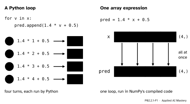
The same four predictions computed two ways. Left: Python visits one value per turn. Right: one expression names the whole array, and the loop runs inside NumPy.
The loop has not disappeared. It has moved. On the left, Python itself walks through the values, and every turn costs Python’s full machinery. On the right, the walk happens inside NumPy, in code that was compiled to machine instructions ahead of time. The NumPy documentation puts it this way: the looping still takes place, “behind the scenes”, in pre-compiled C code.
Machine learning leans on this all the time. A model’s predictions for a whole batch, the errors against the targets and the loss are each one whole-array expression, never a loop over examples.
Build it up
The running data of this lesson are the four points of ML01: inputs x = [1, 2, 3, 4], targets y = [2, 3, 5, 6], and the line \(\hat y = 1.4x + 0.5\). Each step adds one kind of whole-array expression.
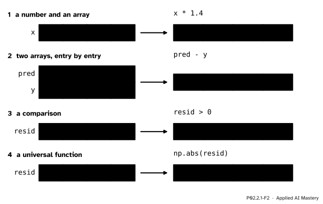
Step 1. A number and an array.x * 1.4 multiplies every entry by 1.4, and x * 1.4 + 0.5 then adds 0.5 to every entry. The result has the same shape as x, here (4,).
Step 2. Two arrays of the same shape.pred - y subtracts entry by entry: the first entry of pred minus the first entry of y, and so on. This course takes a residual as prediction minus target, as ML01 does. The two arrays must have matching shapes; lesson P02.2.3 gives the exact rule.
Step 3. A comparison.resid > 0 compares every entry with 0 and returns an array of True and False of the same shape. It says which points the line overshoots.
Step 4. A universal function. NumPy’s own functions, such as np.sqrt, np.exp and np.abs, also act on every entry. They are called universal functions, or ufuncs.
P02.2.1-F2
Four kinds of whole-array expression. Each one works entry by entry and returns an array of the same shape.
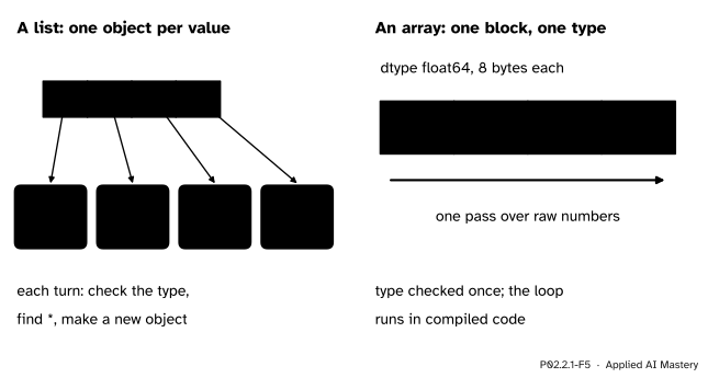
Step 5. Why the array is faster. A Python list does not hold its numbers. It holds a reference to a separate object for each one (P01.6). Each turn of a Python loop fetches that object, checks its type, looks up what * means for that type and builds a brand-new object for the answer. An array holds one block of raw numbers, all of one dtype (P02.1.4). NumPy checks the type once and then runs a tight loop over the block.
P02.2.1-F5
A list points to one object per value; an array is one block of numbers of a single type.
The formal statement
NoteDefinition: element-wise operations
Let a and b be arrays of the same shape, c a number and op one of +, -, *, /, ** or a comparison such as >. Then, at every position i,
(a op b)[i] is a[i] op b[i],
(a op c)[i] is a[i] op c, and (c op a)[i] is c op a[i],
for a universal function f, f(a)[i] is f(a[i]).
The result has the same shape as a. Arithmetic gives numbers and a comparison gives booleans.
The NumPy user guide defines a universal function as one that “operates on ndarrays in an element-by-element fashion”. Every arithmetic operator on arrays is a ufunc too: a + b calls np.add(a, b).
The mean squared error of \(n\) predictions \(\hat y_i\) against targets \(y_i\) is
Read it from the inside out, and each piece is one whole-array step. The difference \(\hat y_i - y_i\) for every \(i\) is pred - y. Squaring every entry is ** 2. The sum divided by \(n\) is .mean(). So the formula becomes one line:
mse = ((pred - y) **2).mean()
Nothing has been approximated: the vectorised line computes exactly the numbers the loop would, because the definition above says that the entry at position i is the loop’s value at turn i.
Go deeper: how much memory a list of numbers really takes
On a typical 64-bit build of Python, a list of \(n\) floats holds \(n\) references of 8 bytes each, and each reference points to a float object that carries, besides its 8-byte value, a count of the references to it and a pointer to its type. sys.getsizeof(1.0) reports 24 bytes on such a build. A float64 array stores just the \(n\) values, 8 bytes each, side by side. So the list takes roughly four times the memory, and, worse for speed, its numbers are scattered wherever the objects happen to live, while the array’s sit in one block that the processor can stream through.
Worked example
Score the line \(\hat y = 1.4x + 0.5\) on the four points.
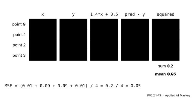
Residuals. Prediction minus target, point by point: \({1.9 - 2 = -0.1}\), \({3.3 - 3 = 0.3}\), \({4.7 - 5 = -0.3}\) and \({6.1 - 6 = 0.1}\).
Squares.\(0.01\), \(0.09\), \(0.09\) and \(0.01\). Their sum is \(0.2\).
Mean.\(0.2 / 4 = 0.05\). So the MSE is \(0.05\).
P02.2.1-F3
The worked example as a trace. Each column is one whole-array step, and each row is one point.
Each column of the trace is one line of NumPy. A loop would fill the table row by row; the vectorised code fills it column by column, one whole column per expression.
Code
First the loop, with plain Python lists, so that every step is visible.
x_list = [1, 2, 3, 4]y_list = [2, 3, 5, 6]pred_list = []for v in x_list: pred_list.append(1.4* v +0.5)resid_list = []for p, t inzip(pred_list, y_list): resid_list.append(p - t)total =0.0for r in resid_list: total = total + r **2mse_loop = total /len(resid_list)print([round(p, 2) for p in pred_list])print([round(r, 2) for r in resid_list])print(round(mse_loop, 4))
The values agree with the loop. The last digits of a float can differ between machines, which is why the checks use np.isclose (P02.1.4) and the printing rounds. np.sqrt(mse) is the root mean squared error, about 0.2236, which is back in the units of \(y\).
Finally, the timing. time.perf_counter() reads a clock meant for measuring short durations; only the difference between two readings means anything. The two versions below do the same work on a million points.
import timerng = np.random.default_rng(0)big_x = rng.uniform(0, 10, size=1_000_000)big_list = big_x.tolist()start = time.perf_counter()out = [1.4* v +0.5for v in big_list]loop_seconds = time.perf_counter() - startstart = time.perf_counter()out_np =1.4* big_x +0.5numpy_seconds = time.perf_counter() - startprint(f"loop: {loop_seconds:.4f} s numpy: {numpy_seconds:.4f} s")
loop: 0.0243 s numpy: 0.0040 s
On a laptop the NumPy line is typically around ten times faster or more, but the exact numbers depend on the Python version, the machine and on what else it is doing, so the lesson prints them and never asserts them. What is checked is that both versions give the same million numbers.
Explore
The interactive of this module, the broadcast stretcher, sits in lesson P02.2.3, once arrays of different shapes have met. Until then, try this: in the Code section, replace 1.4 * x + 0.5 with np.exp(-x) or x ** 2 > 5 and predict the output before you run it.
Pitfalls
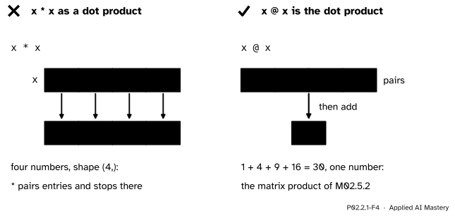
P02.2.1-F4
Wrong beside right. Left:* multiplies matching entries and returns an array. Right:@ multiplies matching entries and then adds them, giving the dot product.
“x * x is the dot product of x with itself.”
* is element-wise: x * x is [1, 4, 9, 16], an array of shape (4,). The dot product, and the matrix product of M02.5.2, is written @: x @ x is 30. Mixing them up gives an array where a number was meant, and a later step may quietly broadcast it into something larger still.
“math.sqrt works on arrays too.”
The functions of the math module take one number. math.sqrt on an array of four entries raises a TypeError. Use the ufunc np.sqrt, which acts on every entry.
“A for loop over an array is as fast as NumPy.”
Looping over an array in Python brings back the per-value cost: each entry is turned into a Python object on every turn, so it is often slower than looping over a list. The speed comes from whole-array expressions, not from storing the data in an array.
“Vectorised code is a different, approximate method.”
It computes exactly what the loop computes, entry by entry. When the two disagree in the last digit, it is because floating-point additions were done in a different order, which is why results are compared with np.isclose, never with ==.
Check yourself
Recall
1. What is vectorisation, in one sentence?
Show answer
Writing an operation once for a whole array, so that the loop over the entries runs inside NumPy instead of in Python.
2. With x = np.array([1, 2, 3, 4]), what is x * 1.4 + 0.5?
Show answer
[1.9, 3.3, 4.7, 6.1], an array of shape (4,).
3. What does resid > 0 return for resid = [-0.1, 0.3, -0.3, 0.1]?
Show answer
An array of booleans of the same shape: [False, True, False, True].
4. Give two reasons why a Python loop over a list of numbers is slower than the NumPy expression.
Show answer
Each turn handles a separate Python object: it checks the type and looks up the operation every time, and builds a new object for each result. NumPy checks the dtype once and loops over one block of raw numbers in compiled code.
5. What is the difference between x * x and x @ x for x = [1, 2, 3, 4]?
Show answer
x * x is element-wise, [1, 4, 9, 16]. x @ x is the dot product, 30.
Exercises
1.★ For the same four points, compute by hand the predictions, residuals and MSE of the line \(\hat y = 1.5x\). Then write the one line of NumPy that gives the MSE.
Show solution
Predictions: \(1.5\), \(3\), \(4.5\), \(6\). Residuals (prediction minus target): \(1.5 - 2 = -0.5\), \(3 - 3 = 0\), \(4.5 - 5 = -0.5\) and \(6 - 6 = 0\). Squares: \(0.25\), \(0\), \(0.25\), \(0\), with sum \(0.5\). MSE \(= 0.5 / 4 = 0.125\), worse than the \(0.05\) of the lesson’s line. In NumPy: ((1.5 * x - y) ** 2).mean(), which gives 0.125.
2.★★ The mean absolute error is the mean of the absolute residuals. Write it first as a loop and then as one NumPy expression, and compute it for the lesson’s line.
Show solution
Loop: total = 0, then for each r in the residuals, total = total + abs(r), and finally total / 4. Vectorised: np.abs(pred - y).mean(). The absolute residuals are \(0.1, 0.3, 0.3, 0.1\), with sum \(0.8\), so the mean absolute error is \(0.8 / 4 = 0.2\).
3.★★★ Without running it, say what np.where(resid > 0, resid, 0) returns for the lesson’s residuals, and explain how it acts entry by entry. Then write the same with a loop. (np.where(mask, a, b) takes a[i] where mask[i] is True and b elsewhere.)
Show solution
The mask resid > 0 is [False, True, False, True]. At each position np.where takes the residual where the mask is True and 0 where it is False, so the result is [0, 0.3, 0, 0.1]: only the overshoots are kept. As a loop: out = [], then for each r, append r if r > 0, else append 0. NumPy runs that same choice over every entry in compiled code.
Summary card
Write the operation once for the whole array; NumPy runs the loop.
P02.2.1-F1
The loop moves inside NumPy.
Element-wise:(a op b)[i] is a[i] op b[i]; a number meets every entry.
Universal functions:np.sqrt, np.exp, np.abs act on every entry.
MSE in one line:((pred - y) ** 2).mean(), which is 0.05 for the four points.
Products:* pairs entries; @ pairs and adds.
Sources and next steps
Sources. Each was opened and checked against this lesson on 15 November 2026.
NumPy developers, What is NumPy?, NumPy user guide, version 2.5. Defines vectorisation as “the absence of any explicit looping, indexing, etc., in the code”, the looping taking place behind the scenes in pre-compiled C code.
NumPy developers, Universal functions (ufunc) basics, NumPy user guide, version 2.5. The definition of a ufunc as a function that operates on arrays element by element.
Jake VanderPlas, Computation on NumPy Arrays: Universal Functions, Python Data Science Handbook. The section “The Slowness of Loops” traces the cost to the type checks and function look-ups that Python makes at every turn of a loop.
Python Software Foundation, time.perf_counter, The Python Standard Library. A clock for short durations, whose reference point is undefined, so that only the difference between two calls is valid.