A group-by on two keys reads best as a grid: one key down the side, the other across the top. Build it with unstack, then with pivot_table and its margins, count pairs with crosstab, see that a confusion matrix is a crosstab, and close on the mean petal length of each iris species.
P02.6.4L1 Core25 minIn review (what this means)
The maths and code on this page are checked by automated tests on every change, but an independent reader has not signed it off yet. Spot a mistake or a confusing step? Tell us.
Lay a two-key group-by out as a grid with unstack and with pivot_table.
Explain what margins=True adds and why a margin is not the mean of the cells beside it.
Count pairs with crosstab, and tell its 0 for an empty pair from the NaN of a mean.
Build a confusion matrix as the crosstab of true labels against predicted labels.
The question
Is a clear sky warmer than a cloudy one at every station, or only on average? The seven rows of a two-key group-by hold the answer, but a list of pairs hides it. Spreadsheet users would build a pivot table: stations down the side, skies across the top, one mean in each cell. The same grid, with counts in the cells, is the confusion matrix that every classifier is judged by.
From the last lesson
1. How does the result of groupby('station')['temp'].transform('mean') differ from that of .mean()?
Show answer
.mean() gives 3 values indexed by station; transform('mean') gives 12 values, one per reading, under the readings’ index 0 to 11.
2. Why is readings['temp'] - readings.groupby('station')['temp'].mean() all NaN?
Show answer
Subtraction matches labels: 0 to 11 on one side and coast, hill, valley on the other. No label has a partner, so all 15 labels get NaN.
Intuition
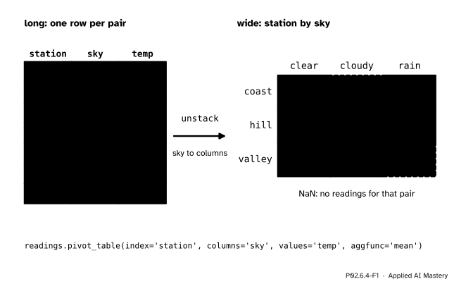
Group by station and sky and you get one row per pair that occurs (lesson P02.6.2). Now move the second key, sky, from the rows to the columns. Each pair becomes a cell of a grid, found by its row and its column, and the grid is read the way a reader’s eye wants to read it: along a row to compare skies at one station, down a column to compare stations under one sky.
P02.6.4-F1
The same seven numbers, long and wide. The grid has nine cells for seven pairs, so the two pairs that never happened show up as NaN.
Two things are easier to see in the grid. Clear is the warmest sky at every station. And the gaps are visible: the valley never saw rain in these four days and the coast never saw a cloudy noon. Wickham names spreadsheet pivot tables as one of the tools that carry out split-apply-combine.
Build it up
Step 1. Group, then unstack.unstack() moves the innermost level of the index, here sky, to the columns:
Every (station, sky) pair finds its cell; a cell with no pair gets NaN.
Step 2. pivot_table does both.pivot_table names the row key, the column key, the value column and the summary in one call, and its summary is the mean unless told otherwise:
It is the pivot of lesson P02.5.3 with an aggregation added. pivot only moves values into place and fails when two rows share a (row, column) pair; pivot_table summarises them.
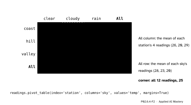
Step 3. Margins.margins=True adds a row and a column labelled All. The All column holds the summary of each whole row key, the All row that of each whole column key, and the corner that of the whole table.
P02.6.4-F2
margins=True. The All column repeats the station means of lesson P02.6.1, the All row the sky means of lesson P02.6.2, and the corner is the overall mean, 25.
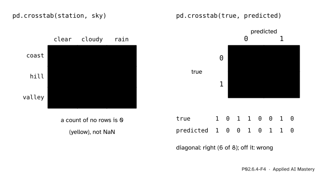
Step 4. Counting pairs.pd.crosstab(rows, columns) counts how many rows fall into each pair: a frequency table. A pair with no rows has the count 0, which is a true statement about a count, where the mean of no values does not exist and is NaN.
P02.6.4-F4
Left: counts of station and sky. Right: the same call on a classifier’s true and predicted labels is its confusion matrix; the diagonal counts the correct answers.
A classifier’s confusion matrix is exactly this. Put the true labels down the side and the predicted labels across the top, and each cell counts one kind of outcome; the diagonal holds the correct ones. Lesson ML01.7.1 reads accuracy, precision and recall off it.
The formal statement
NoteDefinition: pivot table and cross-tabulation
Take a table with a row key \(r\), a column key \(c\) and a value column \(x\), and a summary \(f\). The pivot table has one row per value \(a\) of \(r\) and one column per value \(b\) of \(c\). Its cell is
or NaN when no row has that pair. With margins, the row margin of \(a\) is \(f\) applied to all rows with \({r_i = a}\), the column margin of \(b\) is \(f\) applied to all rows with \({c_i = b}\), and the corner is \(f\) applied to every row. The cross-tabulation is the pivot table of counts, \(n_{ab}\), with 0 where no row has the pair.
A margin of means is weighted by the counts. Write \(m_{ab}\) for the mean in cell \({(a, b)}\) and \(n_{ab}\) for its count from the crosstab. The values in the cell add up to \({n_{ab}\, m_{ab}}\), and the row \(a\) holds \({n_a = \sum_b n_{ab}}\) values in all. So the row margin, the mean of all values in row \(a\), is
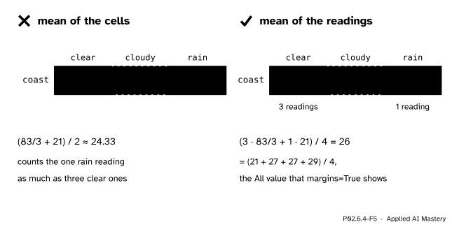
where an empty cell has \({n_{ab} = 0}\) and drops out. This is the weighted mean of lesson P02.6.1 again, now along one row. For the coast, the clear cell holds 3 readings with mean \({83/3}\), about 27.67, and the rain cell 1 reading of 21:
The plain mean of the two cells, \({(27.67 + 21)/2}\), is about 24.33: it counts the single rain reading as much as the three clear ones.
Worked example
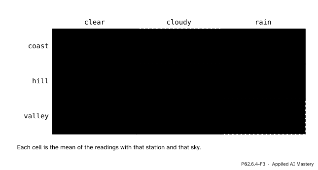
The station-by-sky grid of means, by hand. Go through the nine cells and, for each, collect the readings with that station and that sky.
P02.6.4-F3
The grid filled by hand. Every cell is a small group-by of its own.
Coast. Clear on Tuesday, Wednesday and Thursday: \({(27 + 27 + 29)/3 = 83/3 \approx 27.67}\). Rain on Monday: 21. Never cloudy, so that cell is NaN.
Hill. Clear on Tuesday: 23. Cloudy on Wednesday and Thursday: \({(18 + 20)/2 = 19}\). Rain on Monday: 19.
Valley. Clear on Wednesday and Thursday: \({(30 + 32)/2 = 31}\). Cloudy on Monday and Tuesday: \({(26 + 28)/2 = 27}\). Never rain: NaN.
Read it. Along each row, clear is the warmest sky: 27.67 against 21 at the coast, 23 against 19 at the hill, 31 against 27 at the valley. Check the counts:\({3 + 1 + 1 + 2 + 1 + 2 + 2 = 12}\), every reading in exactly one cell.
Code
The table, then the grid from scratch with a dictionary keyed by pairs:
import numpy as npimport pandas as pdtemps = np.array([[21, 19, 26], [27, 23, 28], [27, 18, 30], [29, 20, 32]])days, stations = ['mon', 'tue', 'wed', 'thu'], ['coast', 'hill', 'valley']readings = pd.DataFrame({'day': [d for d in days for s in stations],'station': stations *4,'temp': temps.ravel(),'sky': ['rain', 'rain', 'cloudy', 'clear', 'clear', 'cloudy','clear', 'cloudy', 'clear', 'clear', 'cloudy', 'clear'],})cells = {}for station, sky, temp inzip(readings['station'], readings['sky'], readings['temp']): cells.setdefault((station, sky), []).append(temp)grid = {s: {k: (sum(cells[(s, k)]) /len(cells[(s, k)]) if (s, k) in cells elseNone)for k in ['clear', 'cloudy', 'rain']} for s in stations}for s in stations:print(s, grid[s])
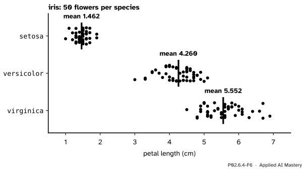
The group-by on real data. Each species is one group of 50 flowers and its mean petal length is one number; no setosa petal is as long as any petal of the other two species, so this one measurement alone separates setosa from them.
Explore
The split-apply-combine machine lives in lesson P02.6.1. Run it with the key station and then with the key sky: the two results are the All column and the All row of this lesson’s pivot table.
Pitfalls
P02.6.4-F5
Wrong beside right. A margin of means weights each cell by its number of readings.
“The All column is the mean of the cells in that row.”
It is the mean of the readings in that row. The coast’s cells, 27.67 and 21, average to about 24.33, but its four readings average to 26, because three of them are clear. The two agree only when every cell holds the same number of readings.
“An empty cell is a zero, so fill it with 0.”
In a table of counts it is: no rows, count 0, which is why crosstab writes 0. In a table of means it is not: fill_value=0 would claim that the valley’s mean in rain was 0 °C. Leave NaN where nothing was measured.
“crosstab(predicted, true) gives the same confusion matrix.”
It gives its transpose: the false positives and the false negatives swap places. Follow one convention and say it; this course puts the true label down the side, as ML01.7.1 does.
“pivot and pivot_table are the same.”
pivot only rearranges and raises an error if a (row, column) pair occurs twice, as (coast, clear) does three times here. pivot_table summarises the repeats with aggfunc.
Check yourself
Recall
1. What does unstack() do to the result of groupby(['station', 'sky'])['temp'].mean()?
Show answer
It moves the inner index level, sky, to the columns, giving a 3 by 3 grid with stations down the side and NaN for the two pairs with no readings.
2. Why does the pivot table of means have NaN for valley in rain while crosstab has 0?
Show answer
There are no such readings. The count of no readings is 0, but the mean of no readings does not exist, so it is missing.
3. What does margins=True add to the pivot table of mean temperature, and what is its corner?
Show answer
An All column with each station’s mean (26, 20, 29), an All row with each sky’s mean (28, 23, 20), and the corner, the mean of all 12 readings, 25.
4. Why is the coast’s All value 26 and not 24.33?
Show answer
It is the mean of the coast’s four readings. The clear cell stands for three of them and the rain cell for one, so they weigh 3 to 1: \({(83 + 21)/4 = 26}\).
5. How do you build a confusion matrix with pandas?
Show answer
pd.crosstab(y_true, y_pred): true labels down the side, predicted labels across, a count in each cell and the correct answers on the diagonal.
Exercises
1.★ Build the pivot table of the highest temperature by station and sky.
Show solution
readings.pivot_table(index='station', columns='sky', values='temp', aggfunc='max') gives coast: clear 29, cloudy NaN, rain 21; hill: clear 23, cloudy 20, rain 19; valley: clear 32, cloudy 28, rain NaN. The cells come from the same collections of readings as the worked example, with the maximum in place of the mean.
2.★★ Build the crosstab of station and sky with margins, then with normalize='index'. What share of the coast’s readings were clear?
Show solution
With margins the body is coast 3, 0, 1; hill 1, 2, 1; valley 2, 2, 0; the All column is 4, 4, 4 and the All row 6, 4, 2, with 12 in the corner. normalize='index' divides each row by its total, so the coast row becomes \({3/4 = 0.75}\), 0 and \({1/4 = 0.25}\): three quarters of the coast’s readings were clear. Every row of shares adds up to 1.
3.★★★ Use the weighted formula with the counts from the crosstab to rebuild the hill’s All value and the clear column’s All value from the cells alone.
Show solution
Hill: the cells are clear 23 from 1 reading, cloudy 19 from 2, rain 19 from 1, so
A pivot table is a two-key group-by laid out as a grid.
P02.6.4-F1
One key down, one key across.
Grid:groupby([r, c])[x].mean().unstack(), or pivot_table(index=r, columns=c, values=x).
Margins:margins=True adds All: each key’s summary over its whole row or column.
A margin of means is the count-weighted mean of its cells, not their plain mean.
Counts:pd.crosstab(r, c), 0 for an empty pair; crosstab(y_true, y_pred) is the confusion matrix.
Sources and next steps
Sources. Each was opened and checked against this lesson on 15 November 2026.
pandas developers, Reshaping and pivot tables, pandas 3.1.1 User Guide: pivot_table for pivoting with aggregation; margins=True adds a row and a column labelled All with partial group aggregates; unstack pivots a level of the row index to the columns; crosstab computes a frequency table of the factors by default.
pandas developers, pandas.pivot_table and pandas.crosstab, pandas 3.1.1 API reference: aggfunc defaults to "mean", margins_name defaults to "All", and the crosstab examples show a count of 0 for a combination that does not occur.
Hadley Wickham, The Split-Apply-Combine Strategy for Data Analysis, Journal of Statistical Software 40(1), 2011. Section 1 names Excel’s pivot tables and the SQL group by operator among the tools that carry out the strategy.
scikit-learn developers, load_iris, scikit-learn 1.9.1: 150 samples in 3 classes of 50, and as_frame=True returns a DataFrame in frame.
Next. P02.7 Dates, text and categories uses time itself as a group key, and ML01.7.1 reads a classifier’s quality off its confusion matrix.