A DataFrame is a dictionary of Series that share one index. Build the weather table by hand and with pd.DataFrame, take a first look with shape, dtypes, head, info and describe, add a column, and reduce along each axis.
P02.4.2L1 Core25 minIn review (what this means)
The maths and code on this page are checked by automated tests on every change, but an independent reader has not signed it off yet. Spot a mistake or a confusing step? Tell us.
Build a DataFrame by hand as a dictionary of Series that share one index, then with pd.DataFrame from an array, row labels and column labels.
Take a first look at any table with shape, dtypes, head, info and describe, and read each output.
Take a column out as a Series and add a new column by assignment with square brackets.
Compute a mean per column and per row, and say which axis each one collapses.
The question
The array temps holds twelve noon readings, but not which station or which day each one belongs to. A spreadsheet would show headings along the top and down the side. What is a table to pandas, and what should you look at first when a new dataset, perhaps the training data of your next model, lands in your hands?
From the last lesson
1. What does coast.loc['tue'] do, step by step?
Show answer
It finds the position of the label 'tue' in the index, 1, and returns the value at that position, 27.
2. Why does coast.std() give 3.464 when np.std gives 3.0?
Show answer
pandas divides the sum of squared distances, 36, by \({n - 1 = 3}\); NumPy divides it by \({n = 4}\).
Intuition
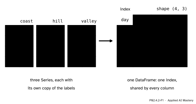
Last lesson’s coast readings were one Series. The hill and valley stations give two more, with the same four days as labels. Stand the three side by side and the labels repeat three times. A DataFrame keeps them once: it is a set of columns, each a Series, that share one index.
P02.4.2-F1
Three Series with the same labels become one DataFrame. The labels are stored once, as the index, and every column lines up against them.
So a DataFrame has labels on both edges. Down the side are the index labels, one per row (the days). Along the top are the column labels, one per column (the stations). The numbers in between are the same twelve as in temps, in the same places: row \(i\), column \(j\).
This is the shape of nearly every dataset in machine learning. Each row is one example (here a day) and each column is one feature (a station’s reading). The data matrix of ML01.1.2, with shape (examples, features), is exactly the grid of numbers inside such a table.
Build it up
Step 1. By hand: a dictionary of Series. A dictionary (P01.6.3) maps each column label to its Series. Asking for a column is a dictionary look-up, and asking for one reading is a column look-up followed by a label look-up.
Step 2. The real thing, two ways.pd.DataFrame accepts that dictionary directly. It also accepts a 2-D array with the labels for each edge, which is how temps from P02.1 becomes a table.
     coast  hill  valley
day
mon     21    19      26
tue     27    23      28
wed     27    18      30
thu     29    20      32
True
The course calls this table wide: one row per day, one column per station. Naming the index day prints that word above the labels; rename_axis(None) takes the name off again for the comparison, and the two tables are equal.
Step 3. The first look. Before computing anything with a new table, look at it. Five tools do most of the work.
P02.4.2-F2
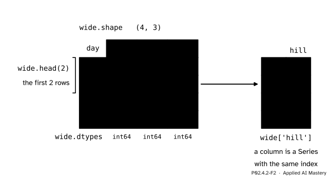
The first look at a table: its shape, the dtype of each column, its first rows, and a column taken out as a Series.
wide.shape is (4, 3): rows first, as for an array.
wide.dtypes gives one dtype per column. Here all three are int64; a real file often mixes numbers with text, whose dtype in pandas 3 is str.
wide.head(n) shows the first n rows (5 if you give no number): the quick look at a table too long to print.
wide.info() prints the index, and for every column its name, how many values are not missing, and its dtype.
wide.describe() prints eight summary numbers for each numeric column. The worked example below computes them by hand.
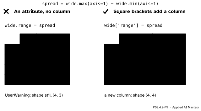
Step 4. Columns in and out.wide['hill'] takes a column out as a Series with the same index. Assigning to a new name in square brackets adds a column, computed for every row at once:
Each day’s range is its highest reading minus its lowest: 7, 5, 12 and 12. The next cells of this lesson start again from the three station columns, after wide = wide.drop(columns='range').
The formal statement
NoteDefinition: DataFrame
A DataFrame with \(n\) rows and \(d\) columns is a set of \(d\) Series that share one index of \(n\) row labels, together with \(d\) column labels, one per Series. Its shape is \({(n, d)}\). Each column has one dtype; different columns may have different dtypes.
Two consequences matter at once.
One index, so rows stay whole. Because every column hangs on the same index, a row is everything the table knows about one label. Sorting or filtering moves whole rows, never one column against the others.
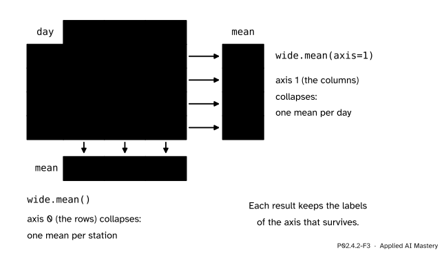
Axes mean what they meant for arrays. A reduction such as mean collapses the axis you name, as in P02.2.2. Axis 0 runs down the rows, so wide.mean() (axis 0 is the default) collapses the rows and leaves one mean per station. Axis 1 runs across the columns, so wide.mean(axis=1) leaves one mean per day.
P02.4.2-F3
A reduction collapses the axis it names. The result is a Series whose index is the labels of the axis that survives: the stations for wide.mean(), the days for wide.mean(axis=1).
The station means are \({104/4 = 26}\), \({80/4 = 20}\) and \({116/4 = 29}\). The day means are \({66/3 = 22}\), \({78/3 = 26}\), \({75/3 = 25}\) and \({81/3 = 27}\). Unlike temps.mean(axis=0), the result knows which number is which: its index is coast, hill, valley.
Worked example
Compute describe() for the coast column by hand.
describe() gives, for each numeric column: count (how many values are not missing), mean, std (dividing by \({n - 1}\), as every pandas std does), min, the quartiles 25%, 50% and 75%, and max. For coast, the first four are 4, 26, 3.464 (from the last lesson) and 21, and the maximum is 29.
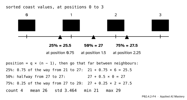
The quartiles need a rule. pandas sorts the values and gives each a position from 0 to \({n - 1}\). The quantile \(q\) sits at position \({q\,(n - 1)}\). When that position falls between two values, it goes the same fraction of the way from the lower value to the upper one; pandas calls this linear interpolation.
P02.4.2-F4
The quartiles of the coast column. Each sits at position \({q(n-1)}\) along the sorted values and is found by going that fraction of the way between its two neighbours.
With \({n = 4}\) the positions run from 0 to 3, and the sorted values are 21, 27, 27, 29.
For the 25% quartile the position is \({0.25 \times 3 = 0.75}\). That lies between position 0 (value 21) and position 1 (value 27), three quarters of the way along, so the quartile is
From scratch first: with the dictionary of Series from Step 1, the station means are one loop over the columns and the day means are one loop over the labels.
station_means = {}for name, column in table.items(): station_means[name] =float(column.sum() /len(column))day_means = {}for day in days: total =0for name in table: total += table[name].loc[day] day_means[day] =float(total /len(table))print(station_means)print(day_means)
The same five tools work on a real dataset. The one this course uses is iris, which ships with scikit-learn: 150 flowers, four measurements each, and a column target with the species as 0, 1 or 2.
from sklearn.datasets import load_irisiris = load_iris(as_frame=True).frameprint(iris.shape)print(iris.dtypes)print(iris['sepal length (cm)'].describe().round(3))
The first look already says a lot: 150 rows, four float columns and one integer column, no missing values, and sepal lengths from 4.3 to 7.9 cm with a mean of 5.843. For a model, the four measurements are the features and target is the label to predict; iris.to_numpy() would give the 150 by 5 grid of numbers underneath.
Explore
This module’s interactive, the label aligner, lives in lesson P02.4.4. It adds two Series whose labels differ, which is where sharing one index starts to matter.
Pitfalls
P02.4.2-F5
Wrong beside right. Assigning to an attribute makes no column; assigning with square brackets does.
“wide.range = spread adds a column called range.”
It does not. A new name after a dot becomes an ordinary Python attribute of the object, and pandas warns with a UserWarning that it does not create columns this way. Reading an existing column as wide.hill works, but it fails for names with spaces, such as iris’ 'sepal length (cm)', and for names that clash with a method (wide.max is the method). Use square brackets for every column.
“axis=1 means one result per column.”
It is the other way round. The axis you name is the one that disappears, so axis=1 collapses the columns and leaves one number per row. Ask “what survives?”: wide.mean() keeps the stations, wide.mean(axis=1) keeps the days.
“wide['hill'] and wide[['hill']] are the same thing.”
One label in square brackets gives a Series of shape (4,). A list of labels gives a DataFrame, even when the list holds one label, of shape (4, 1). The difference is the one between temps[:, 1] and temps[:, 1:2] in P02.3.1, and scikit-learn, which expects a 2-D table of features, needs the second.
Check yourself
Recall
1. What is a DataFrame, in terms of Series?
Show answer
A set of Series, one per column, that share one index, with a label for each column.
2. What does wide.mean(axis=1) return for the weather table?
Show answer
A Series with one mean per day, indexed by the days: 22, 26, 25 and 27. Axis 1, across the columns, is collapsed.
3. Name the five tools of the first look and what each shows.
Show answer
shape (rows and columns), dtypes (the type of each column), head (the first rows), info (index, columns, non-missing counts and dtypes) and describe (count, mean, std, min, quartiles and max of each numeric column).
4. At what position does the 25% quartile of four sorted values sit, and what is it for the coast column?
Show answer
At \({0.25 \times 3 = 0.75}\), three quarters of the way from the first value to the second: \(21 + {0.75 \times 6} = 25.5\).
5. How do you add a column called range to wide?
Show answer
With square brackets: wide['range'] = .... Assigning wide.range = ... makes an attribute, not a column.
Exercises
1.★ Without running code, give wide.shape, wide['valley'].iloc[2], wide.max().to_dict() and wide.max(axis=1).to_dict().
Show solution
wide.shape is (4, 3). wide['valley'].iloc[2] is Wednesday’s valley reading, 30. wide.max() collapses the rows: {'coast': 29, 'hill': 23, 'valley': 32}. wide.max(axis=1) collapses the columns: {'mon': 26, 'tue': 28, 'wed': 30, 'thu': 32}.
2.★★ Compute by hand the three quartiles that describe() gives for the hill column, whose readings are 19, 23, 18 and 20.
Show solution
Sorted: 18, 19, 20, 23 at positions 0 to 3. The 25% quartile sits at 0.75, so it is \(18 + {0.75 \times (19 - 18)} = 18.75\). The median sits at 1.5: \(19 + {0.5 \times (20 - 19)} = 19.5\). The 75% quartile sits at 2.25: \(20 + {0.25 \times (23 - 20)} = 20.75\).
3.★★★ Add a column warmest to wide that holds, for each day, the name of the station with the highest reading, first with a loop over days and stations, then in one line with idxmax. Which station is warmest every day, and why does the one-line version need axis=1?
Show solution
warmest = []for day in days: best = stations[0]for name in stations:if wide[name].loc[day] > wide[best].loc[day]: best = name warmest.append(best)wide['warmest'] = warmest
The one-line version is wide[stations].idxmax(axis=1). idxmax returns the label of the largest value along the axis it collapses; with axis=1 it collapses the stations and returns, for each day, a station label. The valley is warmest on all four days (26, 28, 30 and 32 beat the other two each time). The new column holds text, so wide.dtypes now lists str for it beside the three int64 columns.
Summary card
A DataFrame is a set of Series that share one index.
P02.4.2-F1
Three Series, one shared index.
pd.DataFrame(dict_of_series) or pd.DataFrame(array, index=..., columns=...).
First look: shape, dtypes, head(), info(), describe().
wide['hill'] is a Series; wide['new'] = ... adds a column.
wide.mean() per column, wide.mean(axis=1) per row: the named axis disappears.
Rows are examples and columns are features.
Sources and next steps
Sources. Each was opened and checked against this lesson on 15 November 2026.
pandas development team, Intro to data structures, pandas User Guide, version 3.1.1. The section DataFrame describes it as a two-dimensional labelled structure with columns of potentially different types, like a dict of Series objects.
pandas development team, Essential basic functionality, pandas User Guide, version 3.1.1, section Summarizing data: describe, which lists count, mean, std, min, the quartiles and max for numeric data.
pandas development team, Indexing and selecting data, pandas User Guide, version 3.1.1, section Attribute access: using an attribute to create a new column creates an attribute instead and raises a UserWarning.
pandas development team, pandas.DataFrame.describe and pandas.Series.quantile, API reference, version 3.1.1: the default percentiles are 25, 50 and 75, and the default interpolation is linear between the two neighbouring data points.
scikit-learn developers, load_iris, API reference, version 1.9.1: 150 samples, 3 classes of 50, 4 features, and with as_frame=True a frame of shape (150, 5) holding data and target.