Centre each station’s temperatures on its mean and scale them to standard deviation 1 with two broadcasts, fix the day means with keepdims, and build a table of distances from a column minus a row: the feature scaling and distances of k-nearest neighbours.
P02.2.4L1 Core25 minIn review (what this means)
The maths and code on this page are checked by automated tests on every change, but an independent reader has not signed it off yet. Spot a mistake or a confusing step? Tell us.
Centre the columns of a table with temps - temps.mean(axis=0), and show that every centred column sums to zero.
Standardise each column to mean 0 and standard deviation 1, finishing the coast column by hand.
Repair a failed subtraction of row means with keepdims=True or reshape(4, 1), and explain why it works.
Build the table of distances between points on a line as a column minus a row, and read the nearest neighbour from it.
The question
The valley is always warmer than the hill, so a reading of 23 degrees is a hot day on the hill and a cold one in the valley. How do you put every station on the same footing, so that “unusually warm” means the same thing everywhere? A k-nearest-neighbours model asks the same question of its features, and one line of broadcasting answers it.
From the last lesson
1. What shape does a (4, 3) array combined with a (3,) array give, and why?
Show answer
(4, 3). Lined up from the right, 3 matches 3; the missing axis counts as 1 and is stretched to 4.
2. What does a column (4, 1) minus a row (4,) give?
Show answer
A (4, 4) table, with no error: the column stretches across and the row stretches down.
Intuition
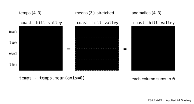
Subtract each station’s mean from its own column. What is left is the anomaly: how much warmer (positive) or cooler (negative) than that station’s usual the reading was. In NumPy it is the expression from the hook of P02.2.3, and the rule of that lesson says why it works: the row of station means, shape (3,), is stretched down the four days.
P02.2.4-F1
Station anomalies. The row of station means is stretched down the days and subtracted; each column of the result sums to 0.
Now the stations can be compared. Thursday was 3 degrees above usual at the coast and the valley, and exactly usual on the hill. Monday was below usual everywhere.
Build it up
Step 1. Centring.temps - temps.mean(axis=0) gives the anomalies in the figure. Centring makes every column average 0: the coast column \({-5 + 1 + 1 + 3}\) sums to 0, and so do the others.
Step 2. The spread of each column. The standard deviation of a column is the square root of the mean squared anomaly. temps.std(axis=0) gives [3, 1.871, 2.236] to three decimals: the coast varies most, the hill least. NumPy divides by \(n\), the number of readings; pandas divides by \(n - 1\) (P02.4.1), which gives 3.464 for the coast instead of 3.
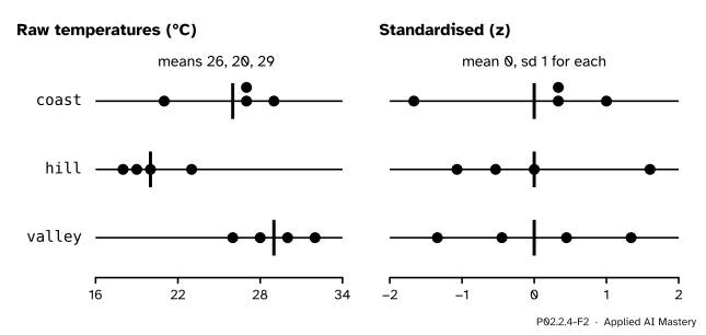
Step 3. Standardising. Divide each anomaly by its column’s standard deviation: (temps - temps.mean(axis=0)) / temps.std(axis=0). Both operations broadcast a row of three numbers down the four days. The results are called z-scores, and every column now has mean 0 and standard deviation 1. This is the feature scaling of ML01.3.3.
P02.2.4-F2
Left: the stations sit at different levels with different spreads. Right: after standardising, each is centred at 0 with a spread of 1, so the dots can be compared directly.
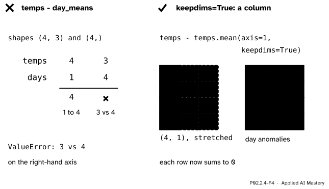
Step 4. The day means need a column. Centring each day instead means subtracting temps.mean(axis=1), shape (4,), which clashes with the 3 stations. Two repairs give the means the shape (4, 1): temps.mean(axis=1, keepdims=True) keeps the collapsed axis (P02.2.2), and temps.mean(axis=1).reshape(4, 1) reshapes afterwards (P02.1.3). Lesson P02.3.1 shows a third spelling, [:, None].
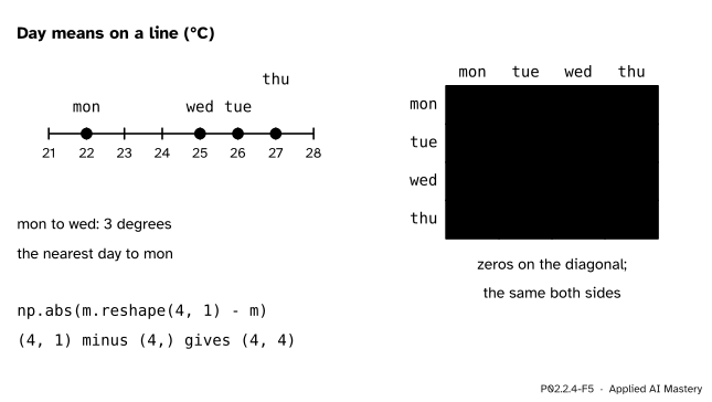
Step 5. A column minus a row. Put the four day means on a line: 22, 26, 25 and 27 degrees. With m holding them, m.reshape(4, 1) - m broadcasts a (4, 1) column against a (4,) row into a (4, 4) table of every difference, and np.abs turns differences into distances. This is the “silent” broadcast of the last lesson’s pitfall, now used on purpose.
P02.2.4-F5
The distances between the four days, computed as a column minus a row. Row mon shows that Wednesday is Monday’s nearest day, 3 degrees away.
The formal statement
NoteDefinition: centring and standardising the columns of a table
Let column \(j\) of a table hold \(x_{1j}, \dots, x_{nj}\). Its mean and its standard deviation (dividing by \(n\)) are
In NumPy, the two numbers per column form rows of shape (3,), and broadcasting stretches them down the rows of the table: (x - x.mean(axis=0)) / x.std(axis=0).
Fact 1: a centred column sums to zero. Drop the index \(j\). Split the sum and use \({\sum_i x_i = n\mu}\):
Fact 2: a standardised column has mean 0 and standard deviation 1. The mean of the \(z_i\) is the mean of the centred values divided by \(\sigma\), which is \(0\) by Fact 1. So the variance of the \(z_i\) is the mean of their squares:
The last step is the definition of \(\sigma^2\). The standard deviation is the square root, also 1. (This needs \(\sigma > 0\): a column whose entries are all equal cannot be standardised.)
Fact 3: the distance table. For points \(m_1, \dots, m_k\) on a line, the table \({D_{ij} = \abs{m_i - m_j}}\) is the column m of shape (k, 1) minus the row m of shape (k,), made positive. It has zeros on its diagonal, since \({\abs{m_i - m_i} = 0}\), and it is symmetric, since \({\abs{m_i - m_j} = \abs{m_j - m_i}}\).
Worked example
Standardise the coast column by hand. The coast readings are 21, 27, 27 and 29.
Anomalies.\({21 - 26 = -5}\), then \(1\), \(1\) and \(3\). They sum to 0, as Fact 1 says.
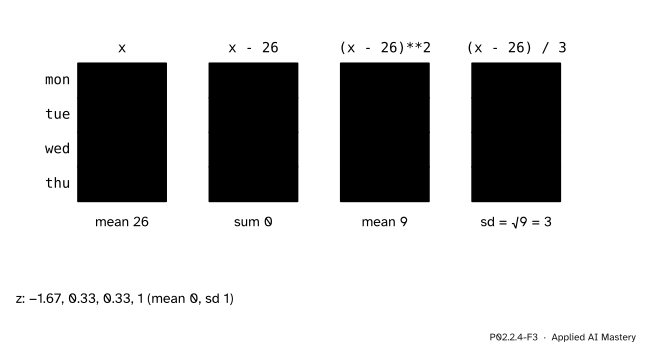
Squares.\(25\), \(1\), \(1\) and \(9\), with sum \(36\). Their mean is \({36 / 4 = 9}\), the variance.
Standard deviation.\({\sqrt{9} = 3}\).
z-scores. Divide each anomaly by 3: \({-5/3 \approx -1.667}\), then \({1/3 \approx 0.333}\) twice, and \({3/3 = 1}\).
P02.2.4-F3
The coast column standardised step by step. The squares have mean 9, so the standard deviation is 3 and each anomaly is divided by 3.
Check Fact 2 on these numbers. The z-scores sum to \({-5/3 + 1/3 + 1/3 + 1 = 0}\). Their squares are \({25/9 + 1/9 + 1/9 + 9/9 = 36/9 = 4}\), and \({4 / 4 = 1}\): mean square 1, so standard deviation 1.
Code
First the station anomalies with loops, then with one broadcast.
The hill’s standard deviation is \({\sqrt{3.5} \approx 1.871}\) and the valley’s \({\sqrt{5} \approx 2.236}\). The column means of z print as 0 and the standard deviations as 1 after rounding; before rounding, the last digits can differ from machine to machine. ddof=1 switches NumPy to dividing by \(n - 1\), which is the 3.464 that pandas reports for the coast.
The day anomalies: the flat means fail, and either repair works.
day_means = temps.mean(axis=1)try: temps - day_meansexceptValueError:print("shapes", temps.shape, "and", day_means.shape, "do not broadcast")by_day = temps - temps.mean(axis=1, keepdims=True)same = temps - day_means.reshape(4, 1)print(by_day)print(np.array_equal(by_day, same), by_day.sum(axis=1))
shapes (4, 3) and (4,) do not broadcast
[[-1. -3.  4.]
 [ 1. -3.  2.]
 [ 2. -7.  5.]
 [ 2. -7.  5.]]
True [0. 0. 0. 0.]
Finally the distance table, and each day’s nearest other day. The diagonal is set to infinity first, so that a day is not its own nearest neighbour; argmin returns the first position on a tie.
Monday’s nearest day is Wednesday (position 2). Tuesday is 1 degree from both Wednesday and Thursday, and argmin picks the first, Wednesday. k-nearest neighbours (ML01.3) does the same with many features at once: the table is built by broadcasting, and every feature is standardised first so that none dominates the distance.
Explore
The broadcast stretcher is in lesson P02.2.3. Pick (4, 3) for A and (4,) for B to see the day means fail, then (4, 1) for B to see the repair stretch across the stations.
Pitfalls
P02.2.4-F4
Wrong beside right. The flat day means (4,) line up with the stations and clash; kept as a column (4, 1) they stretch across the stations and every row is centred.
“The day means are just as easy to subtract as the station means.”
Only once they are a column. temps.mean(axis=1) has shape (4,), which lines up with the 3 stations and fails. Use keepdims=True or reshape(4, 1), and read the shapes before you subtract.
“np.std and pandas’ std give the same number.”
np.std divides by \(n\) by default (ddof=0) and gives 3 for the coast; pandas’ Series.std divides by \(n - 1\) and gives 3.464. Say which one you used. scikit-learn’s StandardScaler divides by \(n\), like NumPy.
“Standardise the whole dataset before splitting it.”
The means and standard deviations are themselves learned from data. Computed on all the rows, they carry information from the test rows into training, the leak of ML01.2.4. Compute them on the training rows only and apply the same two rows of numbers to every other row, as ML01.3.3 does.
“Every column can be standardised.”
A column whose entries are all equal has standard deviation 0, and dividing by it gives nan (0 divided by 0) with a warning. Check stds > 0 first, or drop the constant column: it carries no information anyway.
Check yourself
Recall
1. What are the station anomalies of Thursday?
Show answer
[3, 0, 3]: Thursday’s readings 29, 20, 32 minus the station means 26, 20, 29.
2. Why does every column of temps - temps.mean(axis=0) sum to zero?
Show answer
The sum of \(x_i - \mu\) is \({\sum x_i - n\mu}\), and \({\sum x_i = n\mu}\) by the definition of the mean.
3. What is the standard deviation of the coast column, and what are its z-scores?
Show answer
3, dividing by \(n\). The z-scores are \(-5/3\), \(1/3\), \(1/3\) and \(1\), about \(-1.667\), \(0.333\), \(0.333\), \(1\).
4. Name two ways to make temps - temps.mean(axis=1) work.
Show answer
temps - temps.mean(axis=1, keepdims=True) and temps - temps.mean(axis=1).reshape(4, 1). Both give the day means the shape (4, 1).
5. What shape does m.reshape(4, 1) - m have for m of shape (4,), and what is on its diagonal?
Show answer
(4, 4). Its diagonal holds \({m_i - m_i = 0}\).
Exercises
1.★ Standardise the valley column, 26, 28, 30, 32, by hand.
Show solution
Mean \({116 / 4 = 29}\). Anomalies \(-3\), \(-1\), \(1\), \(3\), which sum to 0. Squares \(9\), \(1\), \(1\), \(9\), with sum \(20\) and mean \(5\), so the standard deviation is \({\sqrt{5} \approx 2.236}\). The z-scores are \({-3/\sqrt{5} \approx -1.342}\), \({-1/\sqrt{5} \approx -0.447}\), \(0.447\) and \(1.342\).
2.★★ Write one NumPy expression that scales each column of temps to run from 0 (its smallest reading) to 1 (its largest), and compute the hill column.
Show solution
(temps - temps.min(axis=0)) / (temps.max(axis=0) - temps.min(axis=0)). Both reductions have shape (3,) and broadcast down the days. For the hill, the minimum is 18 and the maximum 23, a range of 5, so 19, 23, 18 and 20 become \({1/5 = 0.2}\), \(1\), \(0\) and \({2/5 = 0.4}\).
3.★★★ Four points sit on a line at p = [1, 2, 4, 7]. Build the distance table np.abs(p.reshape(4, 1) - p) by hand, find each point’s nearest other point, and say how many different distances between two different points the table can hold at most for \(k\) points, and why.
Show solution
Row by row: [0, 1, 3, 6], [1, 0, 2, 5], [3, 2, 0, 3], [6, 5, 3, 0]. Ignoring the diagonal, the nearest points are: 1 to 2 (distance 1), 2 to 1 (distance 1), 4 to 2 (distance 2) and 7 to 4 (distance 3). The table has \(k^2\) entries, but the \(k\) diagonal ones are 0 and the rest come in equal pairs above and below the diagonal, so it holds at most \({k(k - 1)/2}\) different distances between different points: 6 for \(k = 4\). Here they are 1, 3, 6, 2, 5 and 3, of which 5 are different.
Summary card
Centre with one broadcast, scale with another.
P02.2.4-F1
Anomalies: temps minus station means.
Anomalies: temps - temps.mean(axis=0); each column sums to 0.
Row means need a column: keepdims=True or reshape(4, 1).
Distances: np.abs(m.reshape(4, 1) - m), a (4, 4) table with zeros on the diagonal.
Sources and next steps
Sources. Each was opened and checked against this lesson on 15 November 2026.
NumPy developers, Broadcasting, NumPy user guide, version 2.5. The general rules used here, and the failure for shapes (4,3) and (4,).
NumPy developers, numpy.std and numpy.mean, NumPy reference, version 2.5. std divides by N - ddof with ddof zero by default, and ddof=1 gives the \(n - 1\) version; keepdims=True leaves the reduced axis with size one so that the result broadcasts correctly against the input.
NumPy developers, numpy.argmin, NumPy reference, version 2.5. Notes: with several occurrences of the minimum, the index of the first is returned.
scikit-learn developers, StandardScaler, scikit-learn documentation, version 1.9. Notes: a biased estimator of the standard deviation is used, equivalent to numpy.std(x, ddof=0).
Jake VanderPlas, Computation on Arrays: Broadcasting, Python Data Science Handbook. Section “Centering an array”: subtracting the column means X.mean(0) from a table by broadcasting, and checking that the centred means are near zero.