\( \newcommand{\vect}[1]{\boldsymbol{\mathbf{#1}}} \newcommand{\mat}[1]{\boldsymbol{\mathbf{#1}}} \newcommand{\R}{\mathbb{R}} \newcommand{\E}{\mathbb{E}} \newcommand{\Prob}{\mathbb{P}} \newcommand{\T}{^{\top}} \newcommand{\norm}[1]{\lVert #1 \rVert} \newcommand{\abs}[1]{\lvert #1 \rvert} \newcommand{\ihat}{\mkern1mu\hat{\boldsymbol{\imath}}\mkern2mu} \newcommand{\jhat}{\mkern1mu\hat{\boldsymbol{\jmath}}\mkern2mu} \newcommand{\pd}[2]{\frac{\partial #1}{\partial #2}} \newcommand{\argmax}{\operatorname*{arg\,max}} \newcommand{\argmin}{\operatorname*{arg\,min}} \newcommand{\cdata}[1]{\class{c-data}{#1}} \newcommand{\cmodel}[1]{\class{c-model}{#1}} \newcommand{\ctruth}[1]{\class{c-truth}{#1}} \newcommand{\cgrad}[1]{\class{c-grad}{#1}} \newcommand{\closs}[1]{\class{c-loss}{#1}} \newcommand{\cparam}[1]{\class{c-param}{#1}} \newcommand{\csecond}[1]{\class{c-second}{#1}} \renewcommand{\,}{\mkern3mu} \)

Reshaping: same values, new shape

Reshaping keeps an array’s values in their row-by-row reading order and moves only the row breaks. Derive the flat position k = i * n_cols + j, use reshape, ravel and unravel_index, join arrays with concatenate and stack, and see why reshape is not a transpose.

P02.1.3L1 Core25 min

In review (what this means)

The maths and code on this page are checked by automated tests on every change, but an independent reader has not signed it off yet. Spot a mistake or a confusing step? Tell us.

Before this lesson: P02.1.2 Shape, axes and dimensions

What you will be able to do

• Derive the flat position k = i * n_cols + j of entry [i, j], and recover i and j from k with // and %.
• Rebuild a grid from a flat list with slices, then with reshape, using -1 for the size NumPy can work out.
• Join arrays with np.concatenate along an existing axis and with np.stack along a new one, and predict the result’s shape.
• Tell reshape(3, 4) from the transpose .T by the reading order each one gives.

The question

The weather logger sends the week’s readings as one long line of twelve numbers, 21, 19, 26, 27, 23, 28, 27, 18, 30, 29, 20, 32. How do you turn that line back into the table of four days by three stations, and could the same twelve numbers just as well be three rows of four? Machine learning does this all the time: a 28 by 28 picture of a digit is flattened into 784 numbers for a simple model, and a batch of them is flattened row by row.

From the last lesson

1. What is temps[2, 1], and which axis does the 2 belong to?

Show answer

18. The 2 is the position along axis 0 (row 2, Wednesday); the 1 is along axis 1 (column 1, hill).

2. What is the size of an array of shape (2, 3, 3)?

Show answer

\({2 \times 3 \times 3 = 18}\).

Intuition

Read the table the way you read a page: along row 0 from left to right, then along row 1, and so on. That gives the twelve readings in one line, the reading order of the array (NumPy calls it row-major, or C, order). temps.ravel() returns exactly that line.

Now go the other way. Take the line and cut it after every third value: you get four rows of three, the table. Cut it after every fourth value instead: three rows of four. The values never change places in the line. Only the places where one row ends and the next begins move. That is all a reshape does.

P02.1.3-F1

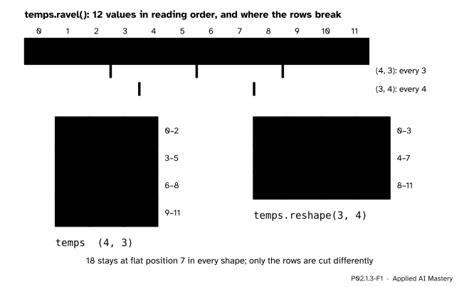
One line of twelve values, cut into rows in two ways. Every value keeps its place in the reading order; reshaping moves only the row breaks.

So a shape is a set of instructions for reading one line of numbers as a grid. Lesson P02.1.1 said an array stores its numbers in one block; this lesson shows how the shape turns a position in the block into a row and a column, and back.

Build it up

Step 1. From a line to a grid, with slices. Cut the line into pieces of three with list slices (P01.6.1): row \(r\) is the slice from \(3r\) up to, but not including, \({3r + 3}\).

flat = [21, 19, 26, 27, 23, 28, 27, 18, 30, 29, 20, 32]
n_cols = 3
grid = [flat[r * n_cols:(r + 1) * n_cols] for r in range(len(flat) // n_cols)]
print(grid)

[[21, 19, 26], [27, 23, 28], [27, 18, 30], [29, 20, 32]]

Step 2. Where entry [i, j] sits in the line. Before row \(i\) come \(i\) full rows of n_cols values each. Inside row \(i\), entry \(j\) has \(j\) values before it. So the number of values before entry \([i, j]\), which is its flat position \(k\), is

\[ k = i \times n_\text{cols} + j . \]

P02.1.3-F2

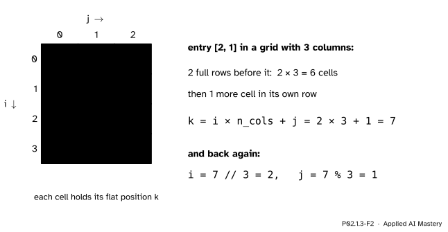
Every cell of a 4 by 3 grid with its flat position written in it. Entry [2, 1] has two full rows (6 cells, orange) and one more cell (green) before it, so its flat position is 7.

Step 3. And back. Given \(k\), the row is the number of full rows that fit before it and the column is what is left over: i = k // n_cols and j = k % n_cols, Python’s floor division and remainder (P01.2.3).

Step 4. The NumPy calls. a.reshape(4, 3) reads a in reading order and cuts it into the new shape; one of the numbers may be -1, meaning “work this one out from the size”. a.ravel() gives the line back, and np.unravel_index(k, shape) turns a flat position into an index.

import numpy as np

line = np.array(flat)
temps = line.reshape(4, 3)
print(temps)
print(line.reshape(3, -1).shape, temps.ravel()[7], np.unravel_index(7, (4, 3)))

[[21 19 26]
 [27 23 28]
 [27 18 30]
 [29 20 32]]
(3, 4) 18 (np.int64(2), np.int64(1))

Step 5. Joining arrays. Two arrays can also be glued into one. np.concatenate joins them along an axis they already have, so that axis grows. np.stack lays them side by side along a brand-new axis, so the result has one more axis than each input.

P02.1.3-F4

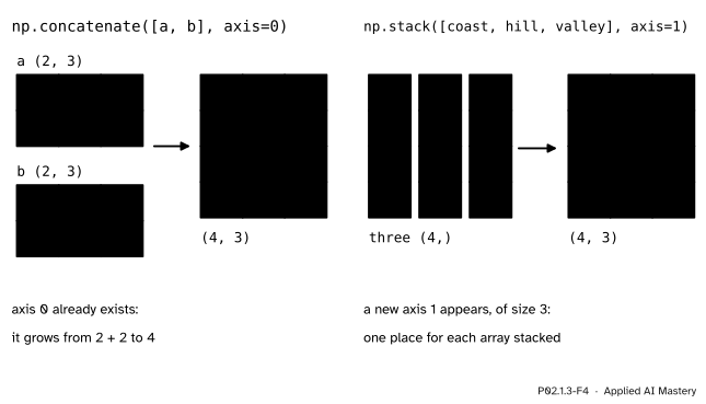
Left: concatenate along axis 0 puts Wednesday and Thursday under Monday and Tuesday. Right: stack along a new axis 1 puts the three station columns side by side.

The formal statement

NoteDefinition: reading order, reshape, transpose

• The flat position of entry \({(i_0, \dots, i_{d-1})}\) of an array of shape \({(n_0, \dots, n_{d-1})}\) is its place in the reading order, in which the last axis changes fastest.
• a.reshape(m0, m1, ...) is allowed exactly when \({m_0 m_1 \cdots}\) equals the size of a. The entry at flat position \(k\) of a goes to flat position \(k\) of the result.
• The transpose a.T reverses the order of the axes. For a 2-D array of shape \({(m, n)}\) it has shape \({(n, m)}\) and a.T[j, i] = a[i, j].

The flat position in any number of dimensions. For two axes, Step 2 gave \({k = i\,n_1 + j}\), where \(n_1\) is the number of columns. Each further axis repeats the argument. For a shape \({(n_0, n_1, n_2)}\), think of the array as \(n_0\) grids of shape \({(n_1, n_2)}\). Before grid \(i_0\) come \(i_0\) whole grids of \(n_1 n_2\) entries each, and inside grid \(i_0\) the entry \({(i_1, i_2)}\) has \({i_1 n_2 + i_2}\) entries before it. Adding the two counts:

\[ \begin{aligned} k &= i_0\,(n_1 n_2) + (i_1\,n_2 + i_2) \\ &= i_0\,n_1 n_2 + i_1\,n_2 + i_2 . \end{aligned} \]

In general each position is multiplied by the product of the sizes of all the axes after it:

\[ k = \sum_{t=0}^{d-1} i_t \prod_{l = t+1}^{d-1} n_l . \]

This is the row-major layout of the NumPy reference, which multiplies each of these products by the number of bytes per entry to find where an entry lives in memory.

Why // and % undo it. Take two axes and \({k = i\,n_1 + j}\) with \({0 \le j < n_1}\). Dividing a whole number \(k\) by \(n_1\) gives exactly one quotient and one remainder with the remainder between 0 and \({n_1 - 1}\). Our \(i\) and \(j\) are such a pair, so they are that quotient and that remainder: \({i = k \,/\!/\, n_1}\) and \({j = k \,\%\, n_1}\). Different indices therefore have different flat positions, and a reshape loses nothing.

What -1 means. In a.reshape(3, -1) the unknown size \(m\) must satisfy \({3m = 12}\), so \({m = 12/3 = 4}\). If the known sizes do not divide the size exactly, as in reshape(5, -1) for 12 values, no whole \(m\) exists and NumPy raises a ValueError. Only one size can be left as -1.

Worked example

Follow the reading 18 from temps into temps.reshape(3, 4), by hand.

P02.1.3-F3

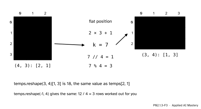
From index [2, 1] of the (4, 3) array to flat position 7, and from there to index [1, 3] of the (3, 4) array.

Into the line. In temps, 18 is at [2, 1] and there are 3 columns, so

\[ k = 2 \times 3 + 1 = 7 . \]

Check against the line 21, 19, 26, 27, 23, 28, 27, 18, ...: counting from 0, position 7 is 18.

Out of the line. The new shape (3, 4) has 4 columns. The row is \({7 \,/\!/\, 4 = 1}\), because one full row of 4 fits before position 7 and two would need 8. The column is \({7 \,\%\, 4 = 3}\), because \({7 - 1 \times 4 = 3}\). So 18 sits at [1, 3] of temps.reshape(3, 4). Check: \({1 \times 4 + 3 = 7}\). Row 1 of the new array is [23, 28, 27, 18]: it holds the last two readings of Tuesday and the first two of Wednesday, because the cut no longer falls between days.

With -1. temps.reshape(-1, 4) asks NumPy for the number of rows: \({12 / 4 = 3}\), the same array.

Into three axes. For temps.reshape(2, 3, 2) the sizes after axis 0 multiply to \({3 \times 2 = 6}\), and after axis 1 to 2. Then \({7 \,/\!/\, 6 = 1}\) with remainder 1, and \({1 \,/\!/\, 2 = 0}\) with remainder 1, so 18 sits at [1, 0, 1]. Check with the formula: \({1 \times 6 + 0 \times 2 + 1 = 7}\).

Code

From scratch: a reshape for two axes that builds the grid entry by entry with the formula, and its inverse.

def my_reshape(values, n_rows, n_cols):
    """Cut a flat list into n_rows rows of n_cols, in reading order."""
    if n_rows * n_cols != len(values):
        raise ValueError("the sizes do not match")
    return [[values[i * n_cols + j] for j in range(n_cols)] for i in range(n_rows)]

def my_unravel(k, n_cols):
    """The [row, column] of flat position k in a grid with n_cols columns."""
    return k // n_cols, k % n_cols

print(my_reshape(flat, 3, 4))
print(my_unravel(7, 3), my_unravel(7, 4))

[[21, 19, 26, 27], [23, 28, 27, 18], [30, 29, 20, 32]]
(2, 1) (1, 3)

The same with NumPy, together with the joins of Step 5 and the transpose:

r = temps.reshape(3, 4)
print(r[1, 3], np.unravel_index(7, (3, 4)), np.unravel_index(7, (2, 3, 2)))

# Monday-Tuesday and Wednesday-Thursday
first, second = np.array(grid[:2]), np.array(grid[2:])
# the three station columns
coast = np.array([row[0] for row in grid])
hill = np.array([row[1] for row in grid])
valley = np.array([row[2] for row in grid])
print(np.concatenate([first, second], axis=0).shape)
print(np.stack([coast, hill, valley], axis=1).shape, np.stack([coast, hill, valley]).shape)
print(temps.T)

18 (np.int64(1), np.int64(3)) (np.int64(1), np.int64(0), np.int64(1))
(4, 3)
(4, 3) (3, 4)
[[21 27 27 29]
 [19 23 18 20]
 [26 28 30 32]]

The pieces are cut from the nested list grid with list slices and comprehensions; lesson P02.3.1 cuts them from the array directly. Stacking the three columns along axis 0 instead of axis 1 gives the transpose: one row per station.

Explore

P02.1-X1

Shape shifter

Choose a shape with the buttons and watch the twelve cells re-flow; the dashed line follows the reading order. Tap a cell, or move the slider, to read its index and its flat position. Then switch on the transpose: which shapes change their reading order, and which one does not?

Pitfalls

P02.1.3-F5

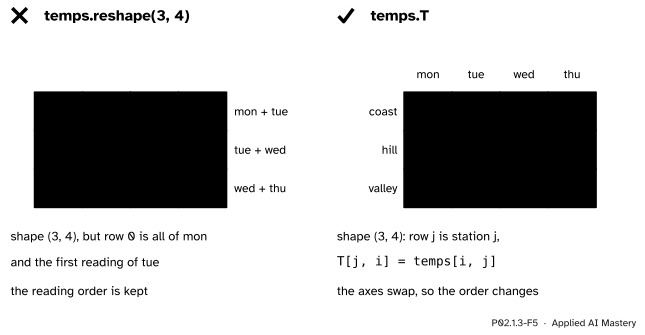
Wrong beside right, when the aim is one row per station. Left: reshape(3, 4) keeps the reading order and cuts the days apart. Right: .T swaps the axes, so each row is one station.

“reshape(3, 4) turns the 4 by 3 table on its side.”

Both give shape (3, 4), but only the transpose turns the table. reshape keeps the reading order, so its first row is Monday’s three readings and the first of Tuesday’s, which means nothing. .T swaps the axes, which changes the reading order: temps.T.ravel() begins 21, 27, 27, 29, the coast column. To swap rows and columns, use .T; to cut the same line differently, use reshape.

“reshape can make any shape I like.”

Only shapes with the same size. temps.reshape(5, 2) asks for 10 places for 12 values and raises a ValueError. With -1, the known sizes must divide the size exactly.

“Flattening a batch: batch.reshape(-1, 784) and batch.reshape(784, -1) are the same.”

A batch of 32 digit images of shape (32, 28, 28) must become (32, 784): one row per image, each image read in its own reading order. batch.reshape(32, -1), or equally batch.reshape(-1, 784), does that. batch.reshape(784, -1) also runs without error, but it gives 784 rows of 32 values: each “example” is a scrap of one image, and some rows run across the end of one image into the next. Always keep the axis of examples first and let -1 stand for the rest.

“concatenate and stack do the same thing.”

concatenate needs the arrays to agree on every axis except the one being joined, and returns the same number of axes. stack needs identical shapes and adds an axis. Concatenating the three station columns of shape (4,) gives one line of 12 values, shape (12,); stacking them gives a (3, 4) or (4, 3) grid.

Check yourself

Recall

1. What is the flat position of entry [i, j] in a grid with n_cols columns?

Show answer

\({k = i \times n_\text{cols} + j}\): the \(i\) full rows before it, plus the \(j\) entries before it in its own row.

2. What does reshaping change, and what does it keep?

Show answer

It keeps the values and their reading order and changes only where the rows break (the shape).

3. What does the -1 in temps.reshape(-1, 4) stand for, and what is it here?

Show answer

The size NumPy works out from the others: \({12 / 4 = 3}\), so the result has shape (3, 4).

4. What is the difference between np.concatenate and np.stack?

Show answer

concatenate joins along an axis the arrays already have, which grows; stack joins along a new axis, so the result has one more axis.

5. temps.reshape(3, 4) and temps.T have the same shape. Why are they different arrays?

Show answer

reshape keeps the reading order 21, 19, 26, 27, …; the transpose swaps the axes, so its rows are the stations and it reads 21, 27, 27, 29, ….

Exercises

1. ★ In temps, what is the flat position of temps[3, 0]? Which index has flat position 5, and what reading is there?

Show solution

\({k = 3 \times 3 + 0 = 9}\), and position 9 of the line is 29, Thursday at the coast. For \({k = 5}\): \({5 \,/\!/\, 3 = 1}\) and \({5 \,\%\, 3 = 2}\), so the index is [1, 2], Tuesday at the valley, 28.

2. ★★ Let a = np.arange(12).reshape(2, 3, 2), so that every entry equals its own flat position. Without running it, find a[0, 2, 1] and the index of the value 10.

Show solution

The sizes after each axis multiply to \({3 \times 2 = 6}\) and 2. So a[0, 2, 1] is \({0 \times 6 + 2 \times 2 + 1 = 5}\). For 10: \({10 \,/\!/\, 6 = 1}\) with remainder 4, and \({4 \,/\!/\, 2 = 2}\) with remainder 0, so 10 is at [1, 2, 0]. Check: \({1 \times 6 + 2 \times 2 + 0 = 10}\).

3. ★★★ Let A have shape \({(m, n)}\). Show that entry \(k\) of A.T.ravel() is A[k % m, k // m], so that the transpose read in order goes down the columns of A. Check it on temps for \({k = 5}\).

Show solution

A.T has shape \({(n, m)}\), so it has \(m\) columns. By Step 3, flat position \(k\) of A.T is its entry [k // m, k % m]. By the definition of the transpose, A.T[j, i] is A[i, j], so with \({j = k \,/\!/\, m}\) and \({i = k \,\%\, m}\) the entry is A[k % m, k // m]. As \(k\) runs through \({0, 1, \dots, m - 1}\) the row \({k \,\%\, m}\) runs through all \(m\) rows while the column stays 0: the first column of A. Then the column becomes 1, and so on. For temps, \({m = 4}\) and \({k = 5}\) give temps[1, 1], which is 23, and temps.T.ravel() is 21, 27, 27, 29, 19, 23, …, whose position 5 is indeed 23.

Summary card

A reshape moves the row breaks; a transpose moves the values.

P02.1.3-F1

Same line, different cuts.

• Flat position. \({k = i \times n_\text{cols} + j}\); back with k // n_cols, k % n_cols.
• Any shape. \({k = \sum_t i_t \prod_{l > t} n_l}\).
• reshape. Same size, same reading order; one size may be -1.
• concatenate / stack. Existing axis grows / new axis appears.
• Transpose. a.T[j, i] = a[i, j]: the reading order changes.

Sources and next steps

Sources. Each was opened and checked against this lesson on 15 November 2026.

• NumPy developers, numpy.reshape, NumPy reference, version 2.5: the new shape must be compatible with the original, one dimension can be -1 and is then inferred, and order ‘C’ reads and writes with the last axis index changing fastest; the result is a view if possible, otherwise a copy.
• NumPy developers, The N-dimensional array (ndarray), NumPy reference, section “Internal memory layout of an ndarray”: the offset of an entry is the sum of its index times the strides, and in row-major (C) order the stride of axis \(k\) is the item size times the product of the sizes of all later axes.
• NumPy developers, numpy.unravel_index, numpy.stack and numpy.ndarray.T, NumPy reference, version 2.5: unravel_index turns flat positions into coordinates in row-major order by default; stack joins arrays of the same shape along a new axis, while concatenate joins along an existing one; .T is the transposed array.

Next. P02.1.4 Data types: what one number can hold looks inside one entry of the block: how many bytes it takes and what it can hold.

This lesson unlocks

P02.1.4 Data types: what one number can hold

Your progress is saved in this browser only. No account, no tracking.