A 2-D array is a grid: the weather table temps has shape (4, 3), ndim 2 and size 12, with axis 0 down the days and axis 1 across the stations. Find a shape by hand, name one entry as temps[i, j], and add a third axis for colour images.
P02.1.2L1 Core25 minIn review (what this means)
The maths and code on this page are checked by automated tests on every change, but an independent reader has not signed it off yet. Spot a mistake or a confusing step? Tell us.
Read the shape, ndim and size of an array, and explain how each follows from the others.
Write shape_of for a rectangular nested list by walking down the first elements.
Name one entry of a 2-D or 3-D array by its index, with axis 0 first, and find it in a grid by hand.
Give the shape of a colour image and of a data matrix, and say what each axis means.
The question
Four days, three stations: twelve readings. To ask for “the valley on Tuesday” you need two numbers, one for the day and one for the station. How does an array know which of its twelve numbers form a row, how many numbers does it take to name one entry, and in which order do they go? In machine learning the same question is asked of every dataset, every image and every batch, and a mix-up between rows and columns is one of the commonest bugs there is.
From the last lesson
1. What does np.array([21, 27]) * 2 give, and what would [21, 27] * 2 give?
Show answer
The array doubles every entry: array([42, 54]). The list repeats itself: [21, 27, 21, 27].
2. How many values does np.arange(26, 33, 2) give?
Show answer
Four, because \({\lceil (33 - 26)/2 \rceil = \lceil 3.5 \rceil = 4}\): 26, 28, 30 and 32.
Intuition
Put the course’s readings side by side: one row per day, one column per station. As nested lists that is four rows of three,
# one row per day (mon to thu), one column per station (coast, hill, valley)temps_list = [[21, 19, 26], [27, 23, 28], [27, 18, 30], [29, 20, 32]]
and np.array(temps_list) turns it into one array, which the course calls temps. The numbers still sit in one block, but the array now also records how to read that block as a grid: 4 rows of 3. That record is the shape, written as a tuple with the rows first: (4, 3).
P02.1.2-F1
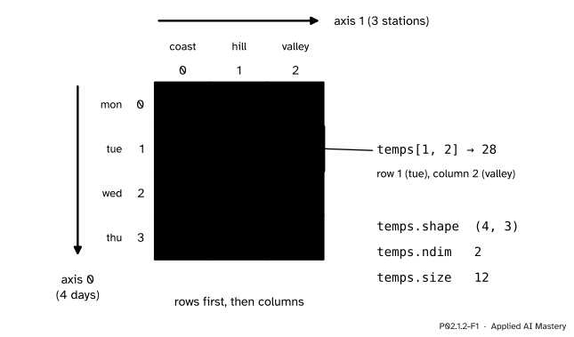
The array temps. Axis 0 runs down the rows (the days) and axis 1 runs across the columns (the stations). One entry is named by one position along each axis, axis 0 first.
Each direction you can move in is an axis. Moving down changes the day: that is axis 0, and it has 4 positions. Moving across changes the station: that is axis 1, with 3 positions. To name one entry you give one position along each axis, in axis order: temps[1, 2] is row 1, column 2, which is Tuesday at the valley, 28 degrees.
The shape says everything about the grid: how many axes there are (its length, 2) and how far each one runs (4 and 3). The day and station names are not stored in the array. Only positions are, and keeping track of what they mean is your job until pandas adds labels in P02.4.
Build it up
Step 1. Two look-ups with lists. With nested lists, a row is one list and an entry is one item of that list, so it takes two look-ups: temps_list[1] is Tuesday’s row [27, 23, 28], and temps_list[1][2] is 28.
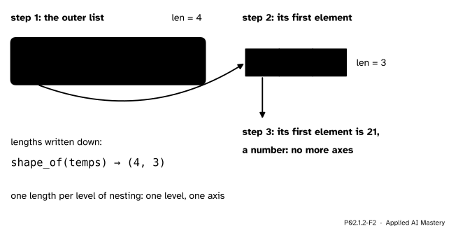
Step 2. Finding the shape by hand. A rectangular nested list hides its shape in its nesting. Walk down it: the outer list has a length, its first element is a list with a length, and so on, until the first element is a number. The lengths written down on the way are the shape.
def shape_of(x):"""The shape of a rectangular nested list, found by walking down the first elements.""" dims = []whileisinstance(x, list): dims.append(len(x))ifnot x: # empty: no first elementbreak x = x[0]returntuple(dims)temps_list = [[21, 19, 26], [27, 23, 28], [27, 18, 30], [29, 20, 32]]print(shape_of(temps_list), shape_of([26, 28, 30, 32]), shape_of(25))
(4, 3) (4,) ()
P02.1.2-F2
shape_of walks down the first elements. Each level of nesting it passes adds one length to the shape; when it reaches a number, it stops.
A plain number has no nesting, so its shape is the empty tuple (). A flat list of four numbers has shape (4,): one axis, written with a comma so that Python reads it as a tuple.
Step 3. The array’s own record. NumPy works the shape out once, when the array is made, and keeps it with the array, along with two numbers that follow from it:
temps.shape is (4, 3);
temps.ndim, the number of axes, is 2, the length of the shape;
temps.size, the number of entries, is 12, the product \({4 \times 3}\).
One pair of square brackets now takes both positions at once, temps[1, 2], and len(temps) gives only the length of axis 0, which is 4.
Step 4. A third axis. Nothing stops at two. A colour image is a grid of pixels, and each pixel holds three numbers: how much red, green and blue it has, each from 0 to 255. So an image of height \(h\) and width \(w\) has shape \({(h, w, 3)}\): a stack of three grids, one per colour, or equally a grid whose every cell holds three numbers.
P02.1.2-F4
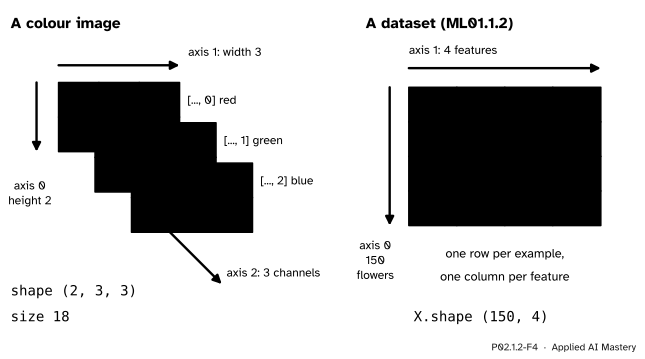
Left: a colour image two pixels high and three wide has shape (2, 3, 3); the third axis picks the colour. Right: the data matrix of lesson ML01.1.2 has one row per example and one column per feature; the iris flowers give (150, 4).
The second picture is the one machine learning uses most. A dataset of \(n\) examples with \(d\) features each is a 2-D array of shape \({(n, d)}\): axis 0 runs over the examples and axis 1 over the features. A batch of images adds an axis in front, (batch, height, width, 3).
The formal statement
NoteDefinition: shape, ndim, size, index
An array with \(d\) axes has a shape\({(n_0, n_1, \dots, n_{d-1})}\), where \(n_k\) is the number of positions along axis \(k\).
Its ndim is \(d\), the length of the shape.
An index is a tuple \({(i_0, i_1, \dots, i_{d-1})}\) of whole numbers with \({0 \le i_k < n_k}\) for every axis \(k\). It names exactly one entry, written a[i0, i1, ...].
Its size is the number of entries, the product of the shape.
Why the size is a product. An entry is named by one index, and an index is a free choice of one position on every axis. There are \(n_0\) choices for \(i_0\). For each of them there are \(n_1\) choices for \(i_1\), which makes \(n_0 n_1\) pairs. For each pair there are \(n_2\) choices for \(i_2\), which makes \(n_0 n_1 n_2\) triples, and so on along all \(d\) axes. Different indices name different entries and every entry has one, so the count of indices is the count of entries.
Three special cases follow from the definition:
ndim 1. Shape \({(n,)}\) has one axis and \(n\) entries; it is neither a row nor a column, just a line of numbers. Shapes \({(n, 1)}\) and \({(1, n)}\) have two axes, and lesson P02.3.1 shows how to move between them.
ndim 0. Shape \({()}\) has no axes. The product of no numbers is 1, so it holds exactly one entry: a single number, such as the result of temps.sum().
Axis order. Axis 0 is always the first number of the shape and the first position of an index. For a 2-D array that is the rows, so a[i, j] is “row \(i\), column \(j\)” (P01.6 counted positions the same way, from 0).
Worked example
Find the shape, ndim and size of temps, and read temps[2, 1], all by hand.
Shape. Walk down temps_list. The outer list has length 4: four days. Its first element, [21, 19, 26], has length 3: three stations. That list’s first element, 21, is a number, so the walk stops. The shape is \({(4, 3)}\).
ndim and size. The shape has two numbers, so ndim is 2. The size is \({4 \times 3 = 12}\), which matches the twelve readings we started with.
One entry.temps[2, 1] asks for position 2 along axis 0 and position 1 along axis 1.
P02.1.2-F3
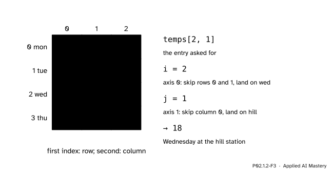
Reading temps[2, 1]: two steps down axis 0 to Wednesday, then one step across axis 1 to the hill station.
Counting from 0, position 2 along axis 0 skips rows 0 and 1 and lands on the third row, Wednesday’s [27, 18, 30]. Position 1 along axis 1 skips column 0 and lands on the second column, the hill station. So temps[2, 1] is 18: the hill station read 18 degrees on Wednesday, the coldest reading of the week.
A third axis. The image in Step 4 has two rows of three pixels with three colours each, so its shape is \({(2, 3, 3)}\), its ndim is 3 and its size is \({2 \times 3 \times 3 = 18}\). The red amount of the pixel in row 0, column 1 is image[0, 1, 0], which is 200; the same pixel’s blue amount is image[0, 1, 2], which is 40.
Code
The worked example, checked with NumPy against the hand-made shape_of:
Finally, a real data matrix. scikit-learn ships the iris measurements with the library, so this runs offline:
from sklearn.datasets import load_irisX, y = load_iris(return_X_y=True)print(X.shape, y.shape, X.ndim, y.ndim)
(150, 4) (150,) 2 1
X has one row per flower and one column per measurement, and y has one label per flower: the shapes \({(n, d)}\) and \({(n,)}\) of lesson ML01.1.2, with \({n = 150}\) and \({d = 4}\).
Explore
This module’s interactive, the shape shifter, lives in lesson P02.1.3. Pick the shape (2, 3, 2) there to see a third axis drawn as a second grid.
Pitfalls
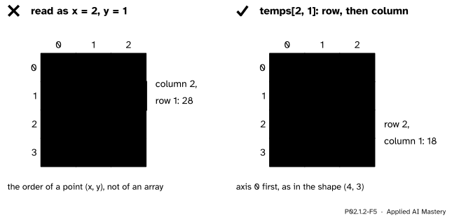
P02.1.2-F5
Wrong beside right. Reading temps[2, 1] like a point \({(x, y)}\) finds 28. The first position is the row, so the entry is 18.
“temps[2, 1] means 2 across and 1 up, like the point (2, 1).”
A point \({(x, y)}\) puts the horizontal position first. An array index puts axis 0 first, and axis 0 runs down the rows. So temps[2, 1] is row 2, column 1, which is 18, not 28. The shape is written the same way: (4, 3) is 4 rows of 3 columns, not 4 wide and 3 tall. An image of shape (480, 640, 3) is 480 pixels high and 640 wide.
“len(temps) is the number of readings.”
len gives the length of axis 0 only, here 4. The number of entries is temps.size, 12. For a dataset X, len(X) is the number of examples, which is often what you want, but not always.
“shape_of tells me the list is a grid.”
shape_of looks only at first elements. For [[1, 2, 3], [4]] it returns (2, 3), yet the second row has one number, not three. Such a list is ragged: no rectangle fits it, and np.array refuses it with a ValueError. Exercise 3 writes the full check.
“Shape (4,) is a column of four numbers.”
It has one axis, so it is neither a row nor a column. A column has shape (4, 1), two axes. The difference matters as soon as two arrays meet in one expression (P02.2.3), so read the shape, not the printout.
Check yourself
Recall
1. What are the shape, ndim and size of temps?
Show answer
Shape (4, 3), ndim 2, size 12.
2. Which way does axis 0 of a 2-D array run, and which way does axis 1 run?
Show answer
Axis 0 runs down the rows (in temps, over the days). Axis 1 runs across the columns (over the stations).
3. What is temps[2, 1], and what does it mean?
Show answer
18: row 2 (Wednesday), column 1 (the hill station).
4. How does the size follow from the shape?
Show answer
It is the product of the numbers in the shape: \({4 \times 3 = 12}\) for temps, and \({2 \times 3 \times 3 = 18}\) for the small image.
5. What shape does a dataset of \(n\) examples and \(d\) features have, and what is axis 0?
Show answer
\({(n, d)}\). Axis 0 runs over the examples, one row each; axis 1 runs over the features.
Exercises
1.★ Give the shape, ndim and size of np.zeros((2, 5)), of np.array([7]), and of the nested list [[[1, 2], [3, 4], [5, 6]]].
Show solution
np.zeros((2, 5)) has shape (2, 5), ndim 2, size 10. np.array([7]) has shape (1,), ndim 1, size 1. For the nested list, walk down: the outer list has length 1, its first element [[1, 2], [3, 4], [5, 6]] has length 3, and its first element [1, 2] has length 2, whose first element is a number. So the shape is (1, 3, 2), ndim 3, size \({1 \times 3 \times 2 = 6}\).
2.★★ A training batch holds 32 colour images, each 64 pixels high and 64 wide. What is the shape of the batch, how many numbers does it hold, and what does axis 3 pick?
Show solution
One image has shape (64, 64, 3), and the batch puts an axis for the 32 images in front: (32, 64, 64, 3). Its size is
Axis 3, the last, has 3 positions and picks the colour: red, green or blue.
3.★★★ Write is_rectangular(x), which returns True exactly when a nested list of numbers can be an array: at every level all the elements are lists of the same length, or all are numbers. Test it on temps_list and on [[1, 2, 3], [4]].
Show solution
A number is a complete block. A list is rectangular when every element is rectangular and all the elements have the same shape, which shape_of from Step 2 can now be trusted to give:
def is_rectangular(x):# a number is a complete blockifnotisinstance(x, list):returnTrue# some element is ragged insideifnotall(is_rectangular(item) for item in x):returnFalse# every element has the same shapereturnlen({shape_of(item) for item in x}) <=1
For temps_list every row is rectangular with shape (3,), so the set of shapes has one member and the answer is True. For [[1, 2, 3], [4]] the shapes are (3,) and (1,), two members, so the answer is False. Comparing whole shapes, not just lengths, also catches [[[1, 2]], [[3]]], whose two elements both have length 1 but shapes (1, 2) and (1, 1). When the function returns True, every element at every level has the shape of the first one, so shape_of gives the true shape.
Summary card
An array’s shape lists how far each axis runs, rows first.
P02.1.2-F1
Axis 0 down, axis 1 across.
Shape.\({(n_0, \dots, n_{d-1})}\); temps is (4, 3).
Index.a[i, j] is row \(i\), column \(j\), with \({0 \le i_k < n_k}\).
Machine learning. Data (n, d); image (h, w, 3); batch in front.
Sources and next steps
Sources. Each was opened and checked against this lesson on 15 November 2026.
NumPy developers, NumPy: the absolute basics for beginners, NumPy user guide, version 2.5. Sections “Array attributes” and “How do you know the shape and size of an array?”: ndim is the number of axes, shape is a tuple giving the number of elements along each dimension, and size is the total number of elements, the product of the elements of the shape.
NumPy developers, The N-dimensional array (ndarray), NumPy reference, version 2.5: an ndarray is a multidimensional container of items of the same type and size, and its shape is a tuple of \(N\) non-negative integers giving the size of each dimension.
scikit-learn developers, sklearn.datasets.load_iris, version 1.9: 150 samples, 3 classes of 50, 4 features; the data matrix has shape (150, 4).