When the rate is a function of t times a function of y, move every y to one side and every t to the other and integrate both. Solve y’ = t y, then logistic growth y’ = y(1 - y), whose solution through (0, 1/2) is exactly the sigmoid, and read stability from the sign of y’.
Recognise a separable equation y’ = g(t) h(y) and solve it by separating the variables and integrating both sides.
Justify separation of variables with the chain rule, and recover the constant solutions that dividing by h(y) loses.
Solve the logistic equation y’ = y(1 - y) with partial fractions, and show that its solution with y(0) = 1/2 is the sigmoid.
Find the equilibria of an autonomous equation y’ = f(y) and decide from the sign of f whether each is stable or unstable.
In review. The maths and code on this page are checked by automated tests on every change, but an independent reader has not signed it off yet. Spot a mistake or a confusing step? Tell us.
The question
Logistic regression turns a score into a probability with the sigmoid, \({\sigma(z) = 1/(1 + e^{-z})}\) (ML01.6), and in M04.3.3 you found its slope: \({\sigma' = \sigma\,(1 - \sigma)}\). Read that identity as a rule about rates. It describes a quantity that grows slowly when it is near 0, fastest in the middle, and slowly again as it nears 1, which is how biologists describe a population that runs out of room. Can you get from the rule back to the formula?
From the last lesson
1. What are all the solutions of \({y' = ky}\)?
Show answer
\({y(t) = y(0)\,e^{kt}}\), and no others.
2. How long does gradient flow on the running loss take to halve its distance to \({47/30}\)?
Show answer
\({\ln 2/15 \approx 0.046}\) units of time, since the distance shrinks like \({e^{-15t}}\).
Intuition
The rule is the logistic equation, \({y' = y\,(1 - y)}\). Here \(y\) is the size of a population as a fraction of what its surroundings can hold. When \(y\) is small there is plenty of room and \({y' \approx y}\), the exponential growth of the last lesson. As \(y\) nears 1 the factor \({1 - y}\) shrinks to nothing and growth stops.
M04.9.3-F1
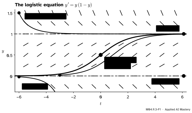
The logistic equation. Every start between 0 and 1 rises along an S to the level 1; the S through \({(0, \frac12)}\) is the sigmoid. Solutions near 1 close in on it, while solutions near 0 move away.
The picture shows two flat lines of dashes, at \({y = 0}\) and at \({y = 1}\). Between them the dashes rise, steepest halfway up, so a solution there climbs along an S. Above 1 and below 0 the dashes fall. So 1 attracts the curves near it and 0 repels them.
Build it up
Step 1. A shape that separates. An equation is separable when its right side is a function of \(t\) times a function of \(y\):
\[
y' = g(t)\,h(y) .
\]
\({y' = t\,y}\) is separable, with \({g = t}\) and \({h = y}\). So is \({y' = y\,(1 - y)}\), with \({g = 1}\). The cooling law \({y' = -k\,(y - c)}\) is too. But \({y' = t + y}\) is not: a sum cannot be written as such a product, and lesson M04.9.4 solves equations like it by small steps.
Step 2. The recipe, on y′ = t y. Write \(y'\) as \({dy/dt}\), divide by \(y\) and multiply by \(dt\), so that every \(y\) is on one side and every \(t\) on the other. Then integrate both sides:
Exponentiate: \({\abs{y} = e^{C}\,e^{t^2/2}}\), so \({y = A\,e^{t^2/2}}\) with \({A = \pm e^C}\). Dividing by \(y\) assumed \({y \neq 0}\), yet \({y = 0}\) is a solution too, since both sides of the equation are then zero. Allowing \({A = 0}\) brings it back, so every solution is \({y = A\,e^{t^2/2}}\). With \({y(0) = 1}\), \({A = 1}\) and \({y = e^{t^2/2}}\). Check:\({y' = t\,e^{t^2/2} = t\,y}\).
Step 3. Why the recipe works. The symbols \(dy\) and \(dt\) are not numbers to be moved about; the recipe is shorthand for the chain rule. Let \(H\) be an antiderivative of \({1/h}\) and \(G\) one of \(g\). If \(y\) solves the equation, the chain rule gives
Two functions with the same derivative differ by a constant (M04.6.3), so \({H(y) = G(t) + C}\): “integrate both sides”. This is the substitution rule of M04.7.1, \({u = y(t)}\), read in reverse.
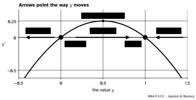
Step 4. Equilibria and their stability. In an autonomous equation \({y' = f(y)}\), a value \(c\) with \({f(c) = 0}\) gives a solution that never moves, \({y = c}\): an equilibrium. Between equilibria \(f\) keeps one sign, and that sign says which way every solution there moves.
M04.9.3-F2
Stability read from the sign of \({y'}\). The arrows point the way \(y\) moves. Both arrows near 1 point at it, so 1 is stable; near 0 they point away, so 0 is unstable.
The formal statement
NoteTheorem: separation of variables
Let \(g\) and \(h\) be continuous, let \(G\) be an antiderivative of \(g\), and let \(H\) be an antiderivative of \({1/h}\) on an interval where \({h \neq 0}\). A differentiable function \(y\) with values in that interval solves \({y' = g(t)\,h(y)}\) exactly when
\[
H\big(y(t)\big) = G(t) + C
\]
for some constant \(C\). Every value \(c\) with \({h(c) = 0}\) gives a further, constant solution \({y = c}\).
Proof. If \(y\) solves the equation, Step 3 shows that \({H(y(t)) - G(t)}\) has derivative zero, so it is a constant \(C\). Conversely, if \({H(y(t)) = G(t) + C}\), differentiate both sides with the chain rule: \({y'/h(y) = g(t)}\), and multiplying by \({h(y)}\) gives back the equation. A constant \({y = c}\) with \({h(c) = 0}\) has \({y' = 0 = g(t)\,h(c)}\). ∎
NoteDefinitions: equilibrium, stable, unstable
For an autonomous equation \({y' = f(y)}\), a value \(c\) with \({f(c) = 0}\) is an equilibrium. It is stable if solutions that start near \(c\) approach \(c\) as \(t\) grows, and unstable if solutions that start arbitrarily near \(c\) are pushed away.
The sign test. Suppose \(f\) is continuous, \({f(c) = 0}\) and no other equilibrium lies close to \(c\). If \({f > 0}\) just below \(c\) and \({f < 0}\) just above, solutions on both sides move towards \(c\), so \(c\) is stable. If the signs are the other way round, solutions move away and \(c\) is unstable. A solution cannot jump over \(c\) on its way, because \({y = c}\) is itself a solution and, for the equations of this module, solution curves do not cross (M04.9.1). For the logistic equation \({f(y) = y\,(1 - y)}\) is positive between 0 and 1 and negative outside, so 1 is stable and 0 is unstable. Stability in general, with several unknowns, is the subject of M12.3.
Go deeper: why a rising solution cannot stall short of the equilibrium
Take \({f > 0}\) on an interval \({(c - \delta, c)}\) and a solution starting there. It rises, and it cannot pass \(c\), so it is an increasing function that stays below \(c\). Such a function has a limit \({\ell \le c}\) as \({t \to \infty}\) (a fact about the real numbers, used here without proof). Suppose \({\ell < c}\). On the closed interval from the start to \(\ell\), \(f\) is positive and continuous, so it has a smallest value \({m > 0}\) there (the extreme value theorem, M04.4.3). Then \({y' \ge m}\) for all time, so \({y(t) \ge y(0) + mt}\), which passes \(c\): a contradiction. So \({\ell = c}\), and the solution closes in on the equilibrium.
Worked example
Solve \({y' = y\,(1 - y)}\) with \({y(0) = \frac12}\).
The start lies between 0 and 1, so the solution stays strictly between them and the division below is allowed.
Separate. Divide by \({y\,(1 - y)}\) and multiply by \(dt\):
\[
\frac{dy}{y\,(1 - y)} = dt .
\]
Split the fraction. Adding the two parts back together confirms the split:
Integrate both sides.\({\int dy/y = \ln y}\), and with the substitution \({u = 1 - y}\), \({du = -dy}\), the second part gives \({\int dy/(1 - y) = -\ln(1 - y)}\). So
\[
\begin{aligned}
\ln y - \ln(1 - y) &= t + C , \\
\ln\frac{y}{1 - y} &= t + C .
\end{aligned}
\]
Exponentiate and solve for y. With \({A = e^C}\), \({y/(1 - y) = A\,e^t}\). Multiply out and collect the terms in \(y\):
Use the start. At \({t = 0}\), \({y/(1 - y) = \frac12/\frac12 = 1}\), so \({A = 1}\). Dividing top and bottom by \({e^t}\),
\[
y = \frac{1}{1 + e^{-t}} = \sigma(t) .
\]
M04.9.3-F3
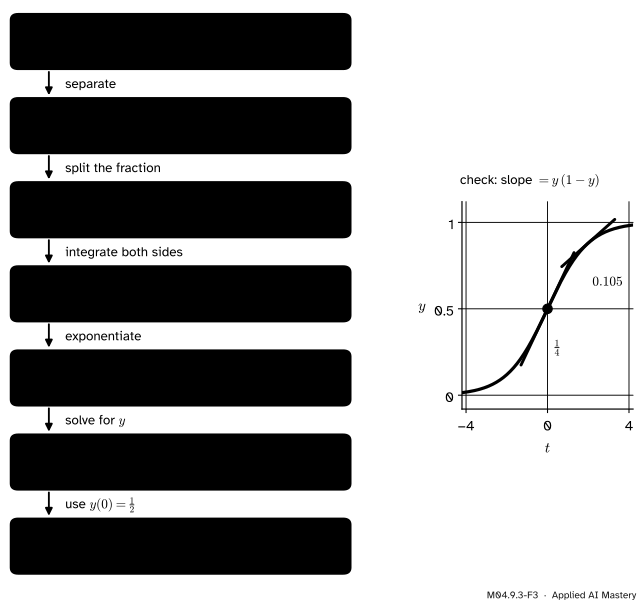
The worked example, one operation per arrow. The check on the right: at every point the sigmoid’s slope is \({y\,(1 - y)}\), a quarter at the middle and 0.105 at \({t = 2}\).
Check. At \({t = 2}\), \({\sigma(2) \approx 0.881}\), and the equation asks for the slope \({0.881 \times 0.119 \approx 0.105}\), which is what \({\sigma'(2)}\) is. Read backwards, the calculation explains M04.3.3: \({\sigma' = \sigma\,(1 - \sigma)}\) because the sigmoid is the solution of the logistic equation.
Any other start between 0 and 1 gives \({A = y(0)/(1 - y(0))}\). From \({y(0) = 0.1}\), \({A = 1/9}\) and \({y = 1/(1 + 9e^{-t})}\), which is \({\sigma(t - \ln 9)}\): the same S, delayed by \({\ln 9 \approx 2.2}\). And on the sigmoid itself, growth from 0.1 to 0.9 takes from \({t = -\ln 9}\) to \({t = \ln 9}\), a span of \({2\ln 9 \approx 4.39}\).
Code
The solution from scratch, checked against the equation by a central difference, and the delayed copy from a start of 0.1:
import mathdef logistic(t, y0):"""The solution of y' = y (1 - y) with y(0) = y0, for 0 < y0 < 1.""" a = y0 / (1- y0)return a * math.exp(t) / (1+ a * math.exp(t))def sigma(z):return1/ (1+ math.exp(-z))h =1e-5for t in (-2.0, 0.0, 2.0): y = logistic(t, 0.5) slope = (logistic(t + h, 0.5) - logistic(t - h, 0.5)) / (2* h)print(f"t = {t:4}: y = {y:.4f}, sigma(t) = {sigma(t):.4f}, slope {slope:.4f}, y(1 - y) = {y * (1- y):.4f}")print("start at 0.1, t = 1:", round(logistic(1.0, 0.1), 6), " sigma(1 - ln 9):", round(sigma(1- math.log(9)), 6))print("from 0.1 to 0.9 on the sigmoid takes", round(2* math.log(9), 3))
t = -2.0: y = 0.1192, sigma(t) = 0.1192, slope 0.1050, y(1 - y) = 0.1050
t =  0.0: y = 0.5000, sigma(t) = 0.5000, slope 0.2500, y(1 - y) = 0.2500
t =  2.0: y = 0.8808, sigma(t) = 0.8808, slope 0.1050, y(1 - y) = 0.1050
start at 0.1, t = 1: 0.231969   sigma(1 - ln 9): 0.231969
from 0.1 to 0.9 on the sigmoid takes 4.394
The sign test for the equilibria, and the separable example \({y' = t\,y}\):
def f(y):return y * (1- y)for c in (0.0, 1.0): below, above = f(c -0.01), f(c +0.01) verdict ="stable"if below >0> above else"unstable"if below <0< above else"neither"print(f"equilibrium {c}: f just below {below:+.4f}, just above {above:+.4f}: {verdict}")y =lambda t: math.exp(t**2/2) # the solution of y' = t y with y(0) = 1print("y' = t y at t = 1.5:", round((y(1.5+ h) - y(1.5- h)) / (2* h), 6), "=", round(1.5* y(1.5), 6))
equilibrium 0.0: f just below -0.0101, just above +0.0099: unstable
equilibrium 1.0: f just below +0.0099, just above -0.0101: stable
y' = t y at t = 1.5: 4.620325 = 4.620325
SciPy names the sigmoid scipy.special.expit. And separation of variables gives the time a solution takes between two values as an integral, \({t = \int dy/f(y)}\), which scipy.integrate.quad can do:
from scipy.integrate import quadfrom scipy.special import expitprint("expit(2) =", round(float(expit(2.0)), 6), " sigma(2) =", round(sigma(2.0), 6))duration, error = quad(lambda v: 1/ (v * (1- v)), 0.1, 0.9)print(f"time from 0.1 to 0.9: {duration:.6f} (2 ln 9 = {2* math.log(9):.6f})")
expit(2) = 0.880797   sigma(2) = 0.880797
time from 0.1 to 0.9: 4.394449   (2 ln 9 = 4.394449)
Explore
The module’s interactive lives in lesson M04.9.4. Choose Logistic, switch Euler’s steps off, and click at different heights: starts between 0 and 1 rise along an S to 1, starts above 1 fall to it, and a start at 0 stays where it is.
Pitfalls
M04.9.3-F4
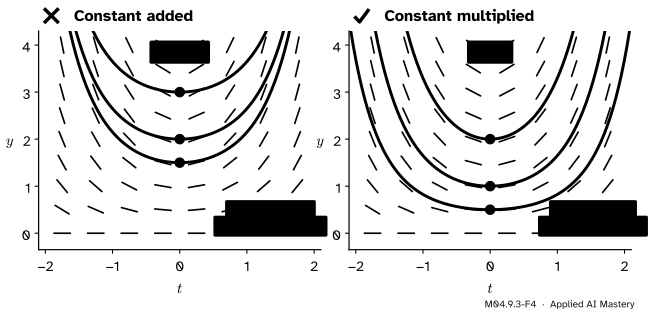
Wrong beside right for \({y' = t\,y}\). Adding a constant after exponentiating shifts the curve and breaks the equation; the constant from integrating becomes a factor, and the scaled copies follow the dashes.
“ln |y| = t²/2 + C, so y = e^(t²/2) + C.”
Exponentiating a sum gives a product: \({e^{t^2/2 + C} = e^C\,e^{t^2/2}}\). The constant becomes a factor, so the solutions are \({A\,e^{t^2/2}}\). The shifted curve \({e^{t^2/2} + 1}\) has slope \({t\,e^{t^2/2}}\), but at its points the equation asks for \({t\,(e^{t^2/2} + 1)}\), more by \(t\).
“Dividing by y(1 − y) is harmless.”
It throws away the solutions \({y = 0}\) and \({y = 1}\), where the divisor is zero. Find the values with \({h(y) = 0}\) first and keep them: they are the equilibria, and the stable one, 1, is where every logistic curve between 0 and 1 ends up.
“An equilibrium is a resting place, so nearby solutions settle there.”
Only a stable one. The logistic equation is at rest at \({y = 0}\), but a start at 0.001 grows away and climbs all the way to 1. Machine learning meets the same distinction: gradient descent can stop at any point where the slope is zero (M04.4.4), but only a minimum draws in the runs that start near it; from beside a maximum, runs move away.
Check yourself
Recall
1. When is a differential equation separable?
Show answer
When its right side is a function of \(t\) times a function of \(y\): \({y' = g(t)\,h(y)}\).
2. Solve \({y' = t\,y}\) with \({y(0) = 3}\).
Show answer
\({y = 3\,e^{t^2/2}}\).
3. How does \({1/(y\,(1 - y))}\) split into two simpler fractions?
Show answer
\({\dfrac{1}{y} + \dfrac{1}{1 - y}}\). Adding them back gives \({\dfrac{(1 - y) + y}{y\,(1 - y)}}\).
4. Which solution of \({y' = y\,(1 - y)}\) is the sigmoid?
Show answer
The one with \({y(0) = \frac12}\): \({y = 1/(1 + e^{-t}) = \sigma(t)}\).
5. Why is \({y = 1}\) a stable equilibrium of the logistic equation?
Show answer
\({y\,(1 - y)}\) is positive just below 1 and negative just above, so solutions on both sides move towards 1.
Exercises
1.★ Solve \({y' = -t\,y}\) with \({y(0) = 1}\). Which curve of this course is the answer?
Show solution
Separate: \({dy/y = -t\,dt}\), so \({\ln\abs{y} = -\tfrac12 t^2 + C}\) and \({y = A\,e^{-t^2/2}}\). The start gives \({A = 1}\): \({y = e^{-t^2/2}}\), the bell curve. Check: \({y' = -t\,e^{-t^2/2} = -t\,y}\). Its values at \({t = 1}\) and 2 are 0.607 and 0.135.
2.★★ Solve \({y' = y\,(1 - y)}\) with \({y(0) = 0.2}\). When does \(y\) reach \({\tfrac12}\), and how fast is it growing then?
Show solution
\({A = 0.2/0.8 = \tfrac14}\), so \({y = \dfrac{1}{1 + 4e^{-t}}}\). It equals \({\tfrac12}\) when \({4e^{-t} = 1}\), at \({t = \ln 4 \approx 1.386}\). There \({y' = \tfrac12 \cdot \tfrac12 = \tfrac14}\), the fastest growth any logistic curve reaches, since \({y\,(1 - y)}\) is largest at \({y = \frac12}\).
3.★★★ The logistic equation with growth rate \({r > 0}\) and carrying capacity\({K > 0}\) is \({y' = r\,y\,(1 - y/K)}\). Solve it for a start \({y_0}\) between 0 and \(K\), find its equilibria and their stability, and find the value of \(y\) at which it grows fastest.
Show solution
Separate and split, using \({\dfrac{1}{y\,(1 - y/K)} = \dfrac{1}{y} + \dfrac{1}{K - y}}\) (add them to check):
with \({A = y_0/(K - y_0)}\). Solving for \(y\) as in the worked example,
\[
y = \frac{K}{1 + \frac{K - y_0}{y_0}\,e^{-rt}} .
\]
The equilibria are the zeros of \({r\,y\,(1 - y/K)}\): 0 and \(K\). The rate is positive between them and negative above \(K\) and below 0, so \(K\) is stable and 0 is unstable. As a function of \(y\) the rate is a downward parabola with roots 0 and \(K\), so it is largest halfway, at \({y = K/2}\), where it equals \({rK/4}\).
Summary card
Separate the variables, integrate both sides, use the start: the logistic equation gives the sigmoid.
M04.9.3-F1
Every S ends at the stable level 1.
Separable.\({y' = g(t)\,h(y)}\) gives \({\int dy/h(y) = \int g(t)\,dt}\), plus the constants where \({h(y) = 0}\).
Example.\({y' = t\,y}\) has the solutions \({A\,e^{t^2/2}}\): the constant multiplies.
Logistic.\({y' = y\,(1 - y)}\) with \({y(0) = \frac12}\) gives \({\sigma(t)}\), so \({\sigma' = \sigma\,(1 - \sigma)}\).
Stability. At an equilibrium of \({y' = f(y)}\), if \({f > 0}\) below and \({f < 0}\) above, it is stable.
Sources and next steps
Sources. Each was opened and checked against this lesson on 12 November 2026.
Gilbert Strang and Edwin Herman, Calculus Volume 2 (OpenStax), Section 4.3: the definition of a separable equation (Equation 4.3) and a five-step strategy whose first step finds the constant solutions where the function of \(y\) is zero. Section 4.4 gives the logistic equation with growth rate \(r\) and carrying capacity \(K\) (Equation 4.8), its constant solutions 0 and \(K\), and its solution (Theorem 4.2) found with the partial fractions \({K/(P(K - P))} = {1/P} + {1/(K - P)}\).
David Jerison, MIT OpenCourseWare 18.01SC, Session 39: Introduction to Differential Equations, with its notes on separation of variables: the form \({dy/dx = f(x)\,g(y)}\), the solution \({y = Ae^{-x^2/2}}\), the solution \({y = 0}\) lost by dividing by \(y\), and the remark that the added constant becomes a multiplied one.
Jiří Lebl, Notes on Diffy Qs, Section 1.6: autonomous equations, equilibria (critical points), stable and unstable equilibria, arrows drawn from the sign of \(f\), and the logistic equation, whose positive equilibrium is stable and whose zero equilibrium is unstable.
Matthew Boelkins, Active Calculus, Section 7.6: the logistic equation (7.6.1), its solution (7.6.2) by partial fractions, and a model population that settles at its carrying capacity.
Next.M04.9.4 Euler’s method follows the slopes in small steps, for the many equations that no formula solves.