A differential equation says how fast a quantity changes in terms of where it is now, and its answer is a whole function. Check a proposed solution by substitution, pick one curve with a starting value, and draw the equation as a field of slopes that every solution follows.
Read a differential equation y’ = f(t, y) as a rule that gives the slope of the unknown function at every point.
Check whether a proposed function solves a differential equation by substitution, and explain why agreement at one point is not enough.
Use an initial condition to pick one solution from a family, as a starting value fixed the constant C in M04.6.3.
Draw the slope field of an equation by hand on a small grid and sketch solution curves through it.
In review. The maths and code on this page are checked by automated tests on every change, but an independent reader has not signed it off yet. Spot a mistake or a confusing step? Tell us.
The question
A thermometer in a cup of tea tells you the temperature now, not in ten minutes. What physics tells you is how fast the tea is cooling: the hotter it is compared with the room, the faster it cools. Training a model is in the same position. The loss says which way a weight should move and how fast, not where it will end up. Can a rule about rates alone pin down a whole curve, and can you see that curve before solving anything?
Intuition
A differential equation is an equation whose unknown is a function, and in which a derivative of that function appears. The kind met in this module gives the slope of an unknown \(y(t)\) at every moment, in terms of the time \(t\) and the present value \(y\):
\[
y' = f(t, y) .
\]
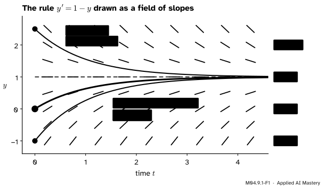
Take \({y' = 1 - y}\). It says nothing about where \(y\) is, only how steeply \(y\) must be moving at each place. Where \({y = -1}\) the slope must be 2; where \({y = 1}\) it must be 0; where \({y = 2}\) it must be \({-1}\). Draw a short dash with the right slope at many points of the plane, and the equation becomes a picture.
M04.9.1-F1
The rule \({y' = 1 - y}\) as a picture. Every dash has the slope the rule demands at its point. A solution is a curve that runs along the dashes; here three solutions from three starts all close in on the line \({y = 1}\).
Three things can be read off the picture before any algebra.
Solutions follow the dashes. A curve that solves the equation has, at each of its points, exactly the slope of the dash there.
Everything heads for the line \({y = 1}\). Below it the dashes climb, above it they fall, and they flatten as they near it.
One start, one curve. A different starting height gives a different solution, but from a given start the dashes leave no choice.
Build it up
Step 1. A rule about rates. Three equations recur in this lesson. In \({y' = 2t}\) the rate depends on the time only. In \({y' = y}\) the rate equals the amount: the more there is, the faster it grows. In \({y' = 1 - y}\) the rate is the distance below 1, like tea cooling towards the room if temperatures are measured so that the room is at 1.
Step 2. The answer is a function. To solve \({y' = 2t}\) we need a function whose derivative is \(2t\). That is an antiderivative (M04.6.3): \({y = t^2 + C}\), and every constant \(C\) works. So a differential equation has a whole family of solutions, not a single number.
Step 3. Check by substitution. To test a proposed solution, work out both sides of the equation and compare them. For the family \({y = 1 + Ce^{-t}}\) and the equation \({y' = 1 - y}\):
The two sides agree for every \(t\), so every member of the family is a solution. The same check shows that \({y = Ce^{t}}\) solves \({y' = y}\), because \({Ce^t}\) is its own derivative (M04.3.2).
Step 4. A starting value picks one curve. Ask for the solution of \({y' = 1 - y}\) with \({y(0) = 0}\). Putting \({t = 0}\) into \({y = 1 + Ce^{-t}}\) gives \({1 + C = 0}\), so \({C = -1}\) and
\[
y = 1 - e^{-t} .
\]
This is the constant \(C\) of M04.6.3 again: there, knowing where the cart started picked one position function out of a family.
Step 5. The slope fields of all three.
M04.9.1-F2
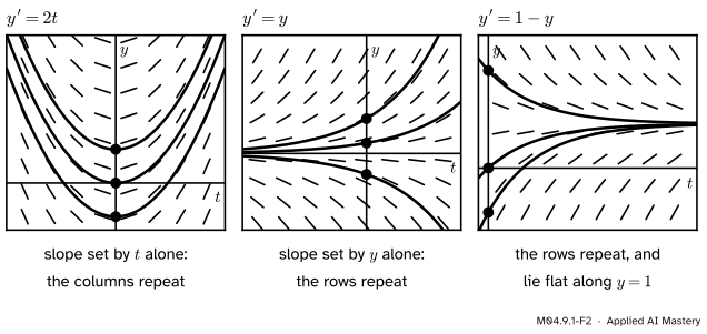
Three rules, three pictures. Where the rate depends on \(t\) alone, the columns of dashes repeat; where it depends on \(y\) alone, the rows repeat.
When the rate depends on \(t\) only, as in \({y' = 2t}\), every dash in a column has the same slope, and the solutions are copies of one parabola shifted up and down. When it depends on \(y\) only, every dash in a row has the same slope, and sliding a solution sideways in time gives another solution.
The formal statement
NoteDefinitions: differential equation, solution, slope field
A first-order differential equation is an equation \({y' = f(t, y)}\) for an unknown function \(y(t)\). A solution on an interval \(I\) is a differentiable function \(y\) such that, for every \(t\) in \(I\),
\[
y'(t) = f\big(t, y(t)\big) .
\]
An initial condition\({y(t_0) = y_0}\) together with the equation is an initial value problem. The slope field of the equation draws, at each point \({(t, y)}\) of a grid, a short segment with slope \({f(t, y)}\).
“First order” means that only the first derivative appears. The spring equation \({y'' = -y}\) is of second order and is left for later courses. When \(f\) involves \(y\) but not \(t\), as in \({y' = y}\) and \({y' = 1 - y}\), the equation is called autonomous.
Why solutions follow the dashes. Suppose \(y\) is a solution whose graph passes through \({(t_1, y_1)}\), so that \({y(t_1) = y_1}\). By the definition, its slope there is
which is the slope of the dash drawn at \({(t_1, y_1)}\). So at every point of a solution curve, the dash is the curve’s tangent line.
Why one start gives one curve. A stronger fact holds for every equation in this module. It is called Picard’s theorem, and its proof belongs to a course on differential equations: if \(f\) is continuous near \({(t_0, y_0)}\), and so is the rate at which \(f\) changes when only \(y\) moves, then exactly one solution passes through \({(t_0, y_0)}\), at least for a while. So two solution curves of such an equation never cross or touch, because at a shared point two different solutions would start from one place. Exercise 3 proves this by hand for \({y' = 1 - y}\).
Go deeper: when two solutions share a start
The condition on \(f\) is not decoration. The equation \({y' = 2\sqrt{\abs{y}}}\) with \({y(0) = 0}\) is solved by \({y = 0}\), since both sides are then zero. It has a second solution: \({y = t^2}\) for \({t \ge 0}\) and \({y = -t^2}\) for \({t < 0}\). For \({t \ge 0}\) the left side is \(2t\) and the right side is \({2\sqrt{t^2} = 2t}\). For \({t < 0}\) the left side is \({-2t}\) and the right side is \({2\sqrt{t^2} = 2\abs{t} = -2t}\). Both sides agree everywhere, so two solutions leave the origin. The rate \({2\sqrt{y}}\) changes infinitely fast as \(y\) leaves 0 (its slope in \(y\), \({1/\sqrt{y}}\), blows up), and that is exactly the condition of Picard’s theorem that fails.
Worked example
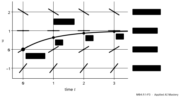
Draw the slope field of \({y' = 1 - y}\) by hand at the sixteen points with \({t = 0, 1, 2, 3}\) and \({y = -1, 0, 1, 2}\). Sketch the solution through \({(0, 0)}\), and check the guess \({y = 1 - e^{-t}}\).
The slopes. The rule does not involve \(t\), so every point of a row gets the same slope:
Row
Slope \({1 - y}\)
The dashes
\({y = 2}\)
\({-1}\)
fall
\({y = 1}\)
\(0\)
lie flat
\({y = 0}\)
\(1\)
rise
\({y = -1}\)
\(2\)
rise twice as steeply
M04.9.1-F3
The worked example. Sixteen dashes, one slope per row, and the curve sketched from \({(0, 0)}\) along them. The marked heights come from the formula \({y = 1 - e^{-t}}\).
The sketch. From \({(0, 0)}\) the curve leaves with slope 1. As it rises, the dashes it meets flatten, so it bends over. It cannot cross \({y = 1}\), which is itself a solution with flat dashes, so it creeps up towards 1.
The check. For \({y = 1 - e^{-t}}\) the left side is \({y' = e^{-t}}\) and the right side is \({1 - (1 - e^{-t})} = {e^{-t}}\). They agree for every \(t\), and \({y(0) = 1 - 1 = 0}\), so this is the solution through \({(0, 0)}\). Its heights at \({t = 1, 2, 3}\) are 0.63, 0.86 and 0.95. The gap to 1, which is \({e^{-t}}\), shrinks by the same factor \({1/e \approx 0.37}\) in each unit of time: 1, 0.37, 0.14, 0.05.
Code
First the slope table from scratch, exactly as by hand.
def f(t, y):"""The rate rule y' = 1 - y: the slope at the point (t, y)."""return1- yfor y in (2, 1, 0, -1):print(f"y = {y:2}:", [f(t, y) for t in (0, 1, 2, 3)])
y =  2: [-1, -1, -1, -1]
y =  1: [0, 0, 0, 0]
y =  0: [1, 1, 1, 1]
y = -1: [2, 2, 2, 2]
Checking a candidate by substitution needs its derivative. A central difference (M04.2.4) measures the slope of any function given as code, so the check becomes a loop over many times.
import mathdef largest_gap(y, f, ts, h=1e-5):"""The largest difference between the slope of y and the slope the equation asks for."""returnmax(abs((y(t + h) - y(t - h)) / (2* h) - f(t, y(t))) for t in ts)times = [k /10for k inrange(31)] # t = 0, 0.1, ..., 3candidates = {"1 - e^(-t)": lambda t: 1- math.exp(-t),"1 - e^(-2t)": lambda t: 1- math.exp(-2* t),"t": lambda t: t,}for name, y in candidates.items():print(f"{name:12} starts at {y(0):.0f}; largest gap {largest_gap(y, f, times):.1e}")print("heights at t = 1, 2, 3:", [round(1- math.exp(-t), 2) for t in (1, 2, 3)])
1 - e^(-t)   starts at 0; largest gap 1.6e-11
1 - e^(-2t)  starts at 0; largest gap 1.0e+00
t            starts at 0; largest gap 3.0e+00
heights at t = 1, 2, 3: [0.63, 0.86, 0.95]
All three candidates start at 0. The line \({y = t}\) even has the right slope at the start, and it fails later, by a gap of 3 at \({t = 3}\). The curve \({y = 1 - e^{-2t}}\) is wrong from the first instant, where it climbs at 2 instead of 1. Only \({1 - e^{-t}}\) passes, with a gap that is rounding error.
The library version uses NumPy arrays. One call computes the slopes on a whole grid, and numpy.gradient measures the slope of sampled values, as it would for data.
import numpy as npT, Y = np.meshgrid([0, 1, 2, 3], [-1, 0, 1, 2]) # rows are y = -1, 0, 1, 2S = f(T, Y) # every slope at onceprint(S)direction = np.array([1, S[0, 0]]) / np.hypot(1, S[0, 0])print("direction of the dash at (0, -1):", np.round(direction, 3))t = np.linspace(0, 3, 3001)y =1- np.exp(-t)slope = np.gradient(y, t, edge_order=2) # the slope of the samplesprint(f"largest gap between the slope and 1 - y: {np.abs(slope - f(t, y)).max():.1e}")
[[ 2  2  2  2]
 [ 1  1  1  1]
 [ 0  0  0  0]
 [-1 -1 -1 -1]]
direction of the dash at (0, -1): [0.447 0.894]
largest gap between the slope and 1 - y: 3.3e-07
The direction \({(1, 2)/\sqrt{5}}\) is a unit arrow with slope 2: a dash is drawn along it. Matplotlib’s quiver draws a whole field of such arrows from arrays like T, Y and S.
Explore
This module’s interactive, the slope field and Euler stepper, lives in lesson M04.9.4. It already works as a slope-field viewer: switch Euler’s steps off with its button, choose an equation, and click anywhere on the field to draw the solution through that point.
Pitfalls
M04.9.1-F4
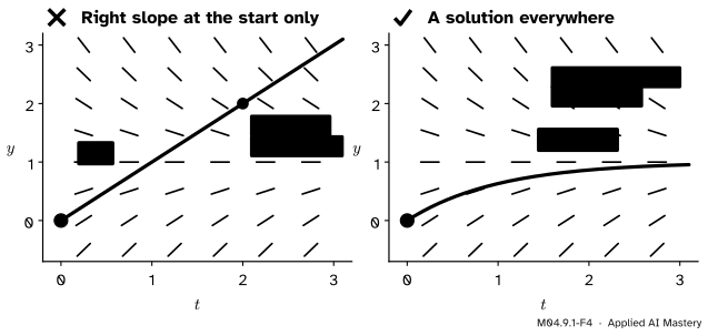
Wrong beside right. The line \({y = t}\) matches the dash at the origin and nowhere else; the true solution through the origin matches every dash it meets.
“It matches at the start, so it is a solution.”
The line \({y = t}\) leaves \({(0, 0)}\) with slope 1, exactly as \({y' = 1 - y}\) asks. At \({t = 2}\) it still climbs at 1, but the rule there asks for \({1 - 2 = -1}\). A solution must obey the rule at every point of its interval. One agreeing point checks one dash.
“Set y′ to zero and solve: the answer is y = 1.”
Solving \({1 - y = 0}\) finds the one solution that never moves, the constant \({y = 1}\). Every other start gives a curve that moves towards it. A differential equation asks for functions, and its constant solutions are only the flat ones among them; lesson M04.9.3 calls them equilibria.
“Two solution curves can cross.”
Not for any equation in this module. Where two curves met, two solutions would leave one point, and Picard’s theorem rules that out. So a solution of \({y' = 1 - y}\) that starts below 1 stays below 1 for ever. The same reasoning tells you, before any computing, that gradient flow on a loss with one lowest point (lesson M04.9.2) can never carry a weight past that point.
Check yourself
Recall
1. What does the equation \({y' = f(t, y)}\) tell you at a point \({(t, y)}\)?
Show answer
The slope that a solution passing through that point must have there: \({f(t, y)}\).
2. How do you check that a function solves a differential equation?
Show answer
Work out its derivative and substitute both into the equation. The two sides must agree at every \(t\) of the interval, not just at one point.
3. Why does \({y' = 2t}\) have infinitely many solutions, and what picks one of them?
Show answer
Every \({y = t^2 + C}\) works, whatever the constant. An initial condition such as \({y(0) = 1}\) fixes \({C = 1}\).
4. In the slope field of \({y' = 1 - y}\), why are all the dashes in a row parallel?
Show answer
The slope \({1 - y}\) depends only on \(y\), so it is the same at every point of a horizontal line.
5. Which constant function solves \({y' = 1 - y}\), and how does it show in the slope field?
Show answer
\({y = 1}\): there the rule gives slope 0, so the dashes along that line lie flat.
Exercises
1.★ Check that \({y = 5e^{2t}}\) solves \({y' = 2y}\). Then find the solution with \({y(0) = 3}\).
Show solution
For \({y = 5e^{2t}}\) the chain rule gives \({y' = 10e^{2t}}\), and \({2y = 10e^{2t}}\): the sides agree for every \(t\). The same check works for \({y = Ce^{2t}}\) with any constant \(C\), because \({y' = 2Ce^{2t} = 2y}\). At \({t = 0}\) this family gives \({y(0) = C}\), so \({C = 3}\) and \({y = 3e^{2t}}\).
2.★★ For \({y' = t - y}\): (a) find the slopes of the dashes at \({(0, 0)}\), \({(1, 0)}\), \({(1, 1)}\) and \({(2, 1)}\); (b) check that \({y = t - 1 + Ce^{-t}}\) is a solution for every \(C\); (c) find the solution through \({(0, 0)}\); (d) find the solution whose graph is a straight line.
Show solution
(a) The slope is \({t - y}\): 0 at \({(0, 0)}\), 1 at \({(1, 0)}\), 0 at \({(1, 1)}\) and 1 at \({(2, 1)}\).
(b) The left side is \({y' = 1 - Ce^{-t}}\). The right side is
\[
\begin{aligned}
t - y &= t - (t - 1 + Ce^{-t}) \\
&= 1 - Ce^{-t} .
\end{aligned}
\]
They agree for every \(t\).
(c) At \({t = 0}\): \({0 - 1 + C = 0}\), so \({C = 1}\) and \({y = t - 1 + e^{-t}}\).
(d) With \({C = 0}\) the solution is the line \({y = t - 1}\). It works because at every point of that line \({t - y = 1}\), which is the slope of the line itself.
3.★★★ Let \(y\) be any solution of \({y' = 1 - y}\) on an interval. Show that \({u(t) = (y(t) - 1)\,e^{t}}\) has derivative zero, and conclude that \({y = 1 + Ce^{-t}}\) for some constant \(C\). Why can two solution curves of this equation never meet?
Show solution
By the product rule (M04.3.3) and the equation \({y' = 1 - y}\),
A function with zero derivative on an interval is constant (M04.6.3), so \({u = C}\), that is \({(y - 1)\,e^{t} = C}\), and \({y = 1 + Ce^{-t}}\). Now suppose two solutions take the same value \(y_1\) at some time \(t_1\). Each has the form \({1 + Ce^{-t}}\), and both constants equal \({(y_1 - 1)\,e^{t_1}}\), so the two solutions are the same function at every time. Two different solution curves therefore never meet.
Summary card
A differential equation gives the slope at every point; a solution is a curve that follows the slopes.
M04.9.1-F1
Dashes give slopes; solutions follow them.
Equation.\({y' = f(t, y)}\); a solution satisfies \({y'(t) = f(t, y(t))}\) at every \(t\).
Check by substituting the function and its derivative, for every \(t\), not one.
Family. Solutions come in families; an initial condition \({y(t_0) = y_0}\) picks one.
Slope field. A dash of slope \({f(t, y)}\) at each point; solution curves are tangent to the dashes and, for the equations here, never cross.
Sources and next steps
Sources. Each was opened and checked against this lesson on 12 November 2026.
Gilbert Strang and Edwin Herman, Calculus Volume 2 (OpenStax), Section 4.1: the definitions of a differential equation, its order and a solution, checking a solution by substitution (Example 4.1), the family \({y = x^2 + C}\) of \({y' = 2x}\) (Figure 4.2) and the initial-value problem. Section 4.2 defines the direction field, which this course calls the slope field, and shows how to draw one.
Matthew Boelkins, Active Calculus, Section 7.2: a slope field as a plot of the tangent lines of many solutions, the fact that a solution through a point is tangent to the line drawn there, and equilibrium solutions of autonomous equations.
Jiří Lebl, Notes on Diffy Qs, Section 1.2: slope fields, Picard’s theorem on existence and uniqueness (Theorem 1.2.1) and Example 1.2.2, in which \({y' = 2\sqrt{\abs{y}}}\) with \({y(0) = 0}\) has two solutions.
Next.M04.9.2 Exponential growth and decay solves \({y' = ky}\) exactly, proves that its solutions are the only ones, and finds the curve that gradient descent follows when its steps become very small.