The tangent line matches a curve’s height and slope; a polynomial of degree n can match its first n derivatives too. Derive the coefficients f^(k)(a)/k!, build e^x, sin x and cos x term by term, and see the line and the parabola that gradient descent and Newton’s method put in place of a loss.
Derive the coefficients f^(k)(a)/k! of the polynomial that matches a function’s value and first n derivatives at a point.
Build the Taylor polynomials of e^x, sin x and cos x at 0 term by term, and recognise the geometric series as those of 1/(1 - x).
Explain a gradient step as trusting T_1 and a Newton step as jumping to the bottom of T_2, and show that T_2 of the running loss is the loss itself.
Evaluate Taylor polynomials from scratch and with numpy.polynomial.Polynomial, and measure their errors.
In review. The maths and code on this page are checked by automated tests on every change, but an independent reader has not signed it off yet. Spot a mistake or a confusing step? Tell us.
The question
The arithmetic a processor does fastest is adding and multiplying, and a polynomial needs nothing more. Yet numpy.exp(0.5) returns 1.64872127…, a value of \({e^x}\). If a polynomial can stand in for \({e^x}\) near 0, which one is it, and how good is it? Asked of a loss near the current weight, the same question is behind every training step: gradient descent treats the loss as a straight line, and Newton’s method treats it as a parabola.
From the last lesson
1. For which \(p\) does \({\sum 1/k^p}\) converge?
Show answer
Exactly for \({p > 1}\).
2. What does the ratio test say when the ratios tend to \({\rho = 1}\)?
Show answer
Nothing: some such series converge, such as \({\sum 1/k^2}\), and some diverge, such as \({\sum 1/k}\).
Intuition
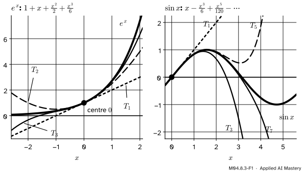
The tangent line of M04.2.2 is the best straight line near a point: it has the curve’s height and slope there. A parabola can match the bend as well, a cubic the way the bend changes, and so on. Each extra term lets the polynomial follow the curve a little further from the point.
M04.8.3-F1
Taylor polynomials building up at the centre 0. Each one matches one more derivative than the last, and follows the curve further out.
These polynomials are the Taylor polynomials of the function about the point, which is called the centre\(a\). The one of degree \(n\) is written \({T_n(x)}\).
Build it up
Step 1. Degree 0: match the value.\({T_0(x) = f(a)}\), a flat line at the right height.
Step 2. Degree 1: match the slope too.\({T_1(x) = f(a) + f'(a)(x - a)}\), the tangent line.
Step 3. Degree 2: match the bend. Add a term \({c_2 (x - a)^2}\). At \({x = a}\) both \({(x - a)^2}\) and its slope \({2(x - a)}\) are 0, so the value and slope still match. Its second derivative is \({2c_2}\), and that of \({T_1}\) is 0, so
Step 4. Degree 3. Add \({c_3 (x - a)^3}\). At \(a\) it and its first two derivatives, \({3(x - a)^2}\) and \({6(x - a)}\), are 0, so nothing already matched is disturbed. Its third derivative is \({6c_3 = 3!\,c_3}\), so \({c_3 = f'''(a)/3!}\).
M04.8.3-F2
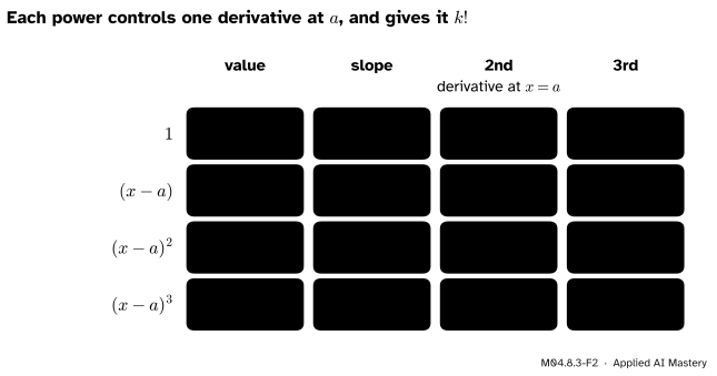
At \({x = a}\) the power \({(x - a)^k}\) has exactly one derivative that is not zero: the \(k\)-th, which is \({k!}\). So the coefficient of \({(x - a)^k}\) controls the \(k\)-th derivative alone.
The pattern is the whole idea. Each power touches one derivative at \(a\), so the coefficients can be chosen one at a time, and the \(k\)-th must be \({f^{(k)}(a)/k!}\).
The formal statement
NoteDefinition: the Taylor polynomial
If \(f\) has \(n\) derivatives at \(a\), its Taylor polynomial of degree \(n\) about \(a\) is
It is the only polynomial of degree at most \(n\) whose value and first \(n\) derivatives at \(a\) equal those of \(f\).
Proof. Any polynomial of degree at most \(n\) can be written in powers of \({x - a}\): put \({x = (x - a) + a}\) into each power of \(x\) and multiply out with the binomial theorem (M01.8). So take \({p(x) = \sum_{k=0}^n c_k (x - a)^k}\). Differentiating \({(x - a)^k}\)\(j\) times gives
when \({j \le k}\), and 0 when \({j > k}\). At \({x = a}\) the factor \({(x - a)^{k-j}}\) is 0 unless \({j = k}\), when it is 1 and the product in front is \({k!}\). So \({p^{(j)}(a) = j!\,c_j}\), and matching \({p^{(j)}(a) = f^{(j)}(a)}\) forces \({c_j = f^{(j)}(a)/j!}\) for every \(j\). That choice does match, so there is exactly one such polynomial. One consequence: a polynomial of degree at most \(n\) is its own \({T_n}\), about any centre, because it matches itself.
Four functions at 0. Every derivative of \({e^x}\) is \({e^x}\), which is 1 at 0. The derivatives of \({\sin x}\) cycle through \({\cos x}\), \({-\sin x}\), \({-\cos x}\) and \({\sin x}\), with values 1, 0, \({-1}\), 0 at 0; those of \({\cos x}\) take the values 0, \({-1}\), 0, 1. For \({1/(1 - x)}\), the chain rule (M04.3.4) applied \(k\) times gives \({k!/(1 - x)^{k+1}}\), which is \({k!}\) at 0. So
\[
\begin{aligned}
e^x &\approx 1 + x + \frac{x^2}{2!} + \frac{x^3}{3!} , \\
\sin x &\approx x - \frac{x^3}{3!} + \frac{x^5}{5!} , \\
\cos x &\approx 1 - \frac{x^2}{2!} + \frac{x^4}{4!} , \\
\frac{1}{1 - x} &\approx 1 + x + x^2 + x^3 .
\end{aligned}
\]
The sine has only odd powers, so its \({T_3}\) and \({T_4}\) are the same polynomial; the cosine has only even powers. The last line is the geometric series of M04.8.1: its Taylor polynomials are its partial sums, and its error is exactly \({x^{n+1}/(1 - x)}\), the gap of M04.8.1.
Two Taylor polynomials that every optimiser uses. About the current weight \({w_t}\) of a loss \(L\),
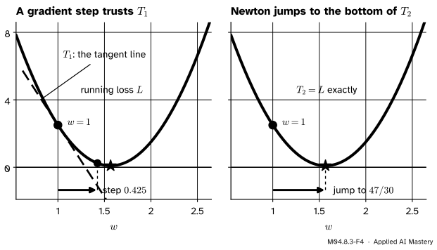
A gradient step moves a short way down the line \({T_1}\), trusting it near \({w_t}\). Newton’s step (M04.4.4) jumps to the lowest point of the parabola \({T_2}\). For the running loss about \({w_t = 1}\): \({L(1) = 2.5}\), \({L'(1) = -8.5}\) and \({L'' = 15}\), so
which is \(L\) itself, as the consequence above promised. That is why Newton’s method lands on \({47/30}\) in one step.
M04.8.3-F4
Two Taylor polynomials of the running loss at \({w = 1}\). A gradient step with \({\eta = 0.05}\) moves 0.425 along \({T_1}\); Newton’s step jumps to the bottom of \({T_2}\), which is the loss itself.
The line promises more than it delivers: along \({T_1}\) the step to 1.425 lowers the loss by \({8.5 \times 0.425 \approx 3.61}\), but the loss falls only to 0.24, by 2.26. The difference, \({7.5 \times 0.425^2 \approx 1.35}\), is exactly the bend term that \({T_2}\) adds.
Worked example
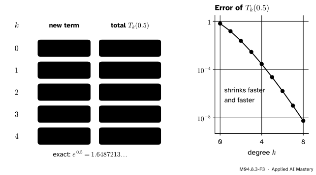
Estimate \({e^{0.5}}\) with \({T_0}\) to \({T_4}\) about 0. Each new term is \({0.5^k/k!}\), which is the term before times \({0.5/k}\):
The worked example as a table: one new term per row and the running total beside it. On the right, the error after each degree falls faster and faster, because each new term is a smaller fraction of the last.
Against \({e^{0.5} = 1.6487213}\), the errors of \({T_0}\) to \({T_4}\) are 0.649, 0.149, 0.0237, 0.00289 and 0.000284. Each error is a little more than the next term, \({0.5^5/5! \approx 0.00026}\) for the last: the terms that were left out add up to not much more than the first of them.
The same way, \({T_3(0.5) = 0.5 - 0.125/6}\), which is 0.4791667, estimates \({\sin 0.5 = 0.4794255}\) with an error of 0.00026; and \({T_4(0.5) = 1 - 0.125 + 0.0026042}\), which is 0.8776042, estimates \({\cos 0.5 = 0.8775826}\) with an error of 0.00002.
Code
From scratch: the coefficients \({f^{(k)}(a)/k!}\), and Horner’s rule, which evaluates a polynomial with one multiplication and one addition per term.
import mathdef taylor_coefficients(derivatives):"""Coefficients f^(k)(a) / k! from the list f(a), f'(a), f''(a), ..."""return [d / math.factorial(k) for k, d inenumerate(derivatives)]def evaluate(coefficients, a, x):"""c_0 + c_1 (x - a) + ... + c_n (x - a)^n, by Horner's rule.""" total =0.0for c inreversed(coefficients): total = total * (x - a) + creturn totalexp_c = taylor_coefficients([1] *13) # every derivative of e^x is 1 at 0sin_c = taylor_coefficients([0, 1, 0, -1, 0, 1]) # sin, cos, -sin, -cos, ... at 0cos_c = taylor_coefficients([1, 0, -1, 0, 1])for n inrange(5):print(f"T_{n}(0.5) = {evaluate(exp_c[:n +1], 0, 0.5):.7f}")print("e^0.5 =", math.exp(0.5), " T_12(0.5) =", evaluate(exp_c, 0, 0.5))print("sin: T_4 =", round(evaluate(sin_c[:5], 0, 0.5), 7), " T_5 =", round(evaluate(sin_c, 0, 0.5), 7)," sin 0.5 =", round(math.sin(0.5), 7))print("cos: T_4 =", round(evaluate(cos_c, 0, 0.5), 7), " cos 0.5 =", round(math.cos(0.5), 7))
The library version is numpy.polynomial.Polynomial, which stores the coefficients from the lowest power up and can be called like a function and differentiated. Here it rebuilds the running loss from its Taylor polynomial at \({w = 1}\):
import numpy as npfrom numpy.polynomial import PolynomialT4 = Polynomial(exp_c[:5]) # 1 + x + x^2/2 + x^3/6 + x^4/24print("T_4(0.5) with Polynomial:", T4(0.5))L = Polynomial([18.5, -23.5, 7.5]) # the running loss 18.5 - 23.5 w + 7.5 w^2d0, d1, d2 = L(1.0), L.deriv()(1.0), L.deriv(2)(1.0) # L(1), L'(1), L''(1)s = Polynomial([-1.0, 1.0]) # the power (w - 1)T2 = d0 + d1 * s + d2 /2* s**2print("L(1), L'(1), L''(1):", d0, d1, d2)print("T_2 about 1, multiplied out:", T2.coef)print("Newton's step from 1:", 1- d1 / d2, " 47/30 =", 47/30)w1 =1-0.05* d1print("drop promised by T_1:", round(-d1 * (w1 -1), 4), " actual drop:", round(L(1.0) - L(w1), 4))
T_4(0.5) with Polynomial: 1.6484375
L(1), L'(1), L''(1): 2.5 -8.5 15.0
T_2 about 1, multiplied out: [ 18.5 -23.5   7.5]
Newton's step from 1: 1.5666666666666667    47/30 = 1.5666666666666667
drop promised by T_1: 3.6125   actual drop: 2.2578
Explore
M04.8-X1
Taylor builder
Choose a function, then step the degree up from 0 and watch each polynomial hug the curve further out; drag the probe to read the error anywhere. For \({\ln(1 + x)}\) and \({1/(1 - x)}\), put the probe beyond 1 and raise the degree: there, more terms end up making things worse.
Pitfalls
M04.8.3-F5
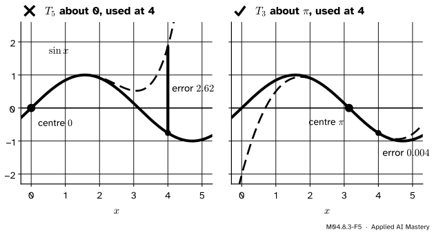
Wrong beside right. \({T_5}\) about 0 is excellent near 0 and useless at 4. A polynomial of lower degree, \({T_3}\) about \({\pi}\), is within 0.004 of \({\sin 4}\), because its centre is close.
“A higher degree is always better, wherever it is used.”
A Taylor polynomial is built from what happens at its centre. Far away, a higher degree can even be worse: at \({x = 4}\), \({T_1}\) of \({\sin x}\) about 0 misses by 4.76 and \({T_3}\) by 5.91. To use a Taylor polynomial at a point, centre it near that point.
“The coefficients are the derivatives.”
They are the derivatives divided by \({k!}\). Without the factorials, \({1 + x + x^2 + x^3}\) is the \({T_3}\) of \({1/(1 - x)}\), a different function: at 0.5 it gives 1.875, against \({e^{0.5} \approx 1.6487}\).
“A Taylor polynomial is always taken at 0.”
Any centre where the derivatives exist will do, and the best centre is near where the polynomial will be used. In training it is the current weight. Some functions have no Taylor polynomial at 0 at all: \({\ln x}\) is not even defined there, but about 1 it gives \({(x - 1) - (x - 1)^2/2 + \cdots}\).
Check yourself
Recall
1. What does \({T_n}\) about \(a\) share with \(f\)?
Show answer
Its value and its first \(n\) derivatives at \(a\).
2. What is the coefficient of \({(x - a)^k}\) in \({T_n}\), and where does the \({k!}\) come from?
Show answer
\({f^{(k)}(a)/k!}\). The \(k\)-th derivative of \({(x - a)^k}\) is \({k!}\), so the coefficient must be divided by it.
3. Write \({T_4}\) of \({\cos x}\) about 0.
Show answer
\({1 - x^2/2 + x^4/24}\).
4. Why is \({T_4 = T_3}\) for \({\sin x}\) about 0?
Show answer
The coefficient of \({x^4}\) is \({\sin(0)/4! = 0}\): the sine has only odd powers.
5. Which Taylor polynomial does a gradient step trust, and which one does Newton’s method jump to the bottom of?
Show answer
A gradient step trusts the line \({T_1}\); Newton’s method jumps to the lowest point of the parabola \({T_2}\).
Exercises
1.★ Find \({T_2}\) of \({\sqrt{x}}\) about 4, use it to estimate \({\sqrt{4.1}}\), and compare with the tangent-line estimate 2.025 of M04.2.2.
Show solution
\({f(4) = 2}\); \({f'(x) = 1/(2\sqrt{x})}\), so \({f'(4) = 1/4}\); \({f''(x) = -1/(4x^{3/2})}\), so \({f''(4) = -1/32}\). Then
The true value is 2.0248457, so the error falls from about 0.00015 for \({T_1}\) to about 0.000002.
2.★★ Find \({T_3}\) of \({\ln(1 + x)}\) about 0 and use it to estimate \({\ln 1.1}\).
Show solution
The derivatives are \({1/(1 + x)}\), \({-1/(1 + x)^2}\) and \({2/(1 + x)^3}\), with values 1, \({-1}\) and 2 at 0, and \({\ln 1 = 0}\). Dividing by \({1!}\), \({2!}\) and \({3!}\): \({T_3(x) = x - x^2/2 + x^3/3}\). So \({\ln 1.1 \approx 0.1 - 0.005 + 0.000333}\), which is 0.0953333, against the true 0.0953102.
3.★★★ Show that a polynomial of degree at most \(n\) equals its own \({T_n}\) about every centre, and use it to write \({x^3}\) in powers of \({x - 1}\).
Show solution
A polynomial \(p\) of degree at most \(n\) has the same value and first \(n\) derivatives at \(a\) as itself, and by the result \({T_n}\) is the only polynomial of degree at most \(n\) with that property, so \({T_n = p}\). For \({p(x) = x^3}\) about 1: \({p(1) = 1}\), \({p'(1) = 3}\), \({p''(1) = 6}\) and \({p'''(1) = 6}\), so
which is the binomial theorem applied to \({\big((x - 1) + 1\big)^3}\).
Summary card
Match the value and the first \(n\) derivatives at the centre, and the coefficients must be \({f^{(k)}(a)/k!}\).
M04.8.3-F1
Taylor polynomials building up.
\({T_n(x)}\) adds up \({f^{(k)}(a)(x - a)^k / k!}\) for \({k = 0, \dots, n}\).
At 0: \({e^x \approx 1 + x + x^2/2! + \cdots}\), \({\sin x \approx x - x^3/3! + \cdots}\), \({\cos x \approx 1 - x^2/2! + \cdots}\), \({1/(1 - x) \approx 1 + x + x^2 + \cdots}\).
A polynomial of degree at most \(n\) is its own \({T_n}\).
In training: a gradient step trusts \({T_1}\); Newton jumps to the bottom of \({T_2}\).
Sources and next steps
Sources. Each was opened and checked against this lesson on 12 November 2026.
Marc Peter Deisenroth, A. Aldo Faisal and Cheng Soon Ong, Mathematics for Machine Learning, Section 5.1.1: the Taylor polynomial \({T_n}\) (Definition 5.3, equation 5.7) and series (Definition 5.4), the remark that a Taylor polynomial of degree \(n\) is exact for a polynomial of degree at most \(n\) (Example 5.3 shows it for \({x^4}\)), and the polynomials of \({\sin x + \cos x}\) in Example 5.4 and Figure 5.4.
Gilbert Strang and Edwin Herman, Calculus Volume 2 (OpenStax), Section 6.3: the definition of the Taylor polynomial, and the Maclaurin polynomials of \({e^x}\), \({\sin x}\) and \({\cos x}\) in Example 6.12, where \({p_{2m+1} = p_{2m+2}}\) for the sine.
Matthew Boelkins, Active Calculus, Section 8.2: Taylor polynomials defined as the polynomials that match the value and first \(n\) derivatives at the centre (Definitions 8.2.3 and 8.2.17), and the coefficients \({f^{(k)}(a)/k!}\) found in the results that follow each definition.
NumPy developers, numpy.polynomial.Polynomial (NumPy 2.5 reference): coefficients in order of increasing degree, deriv, and evaluation by calling the object.