The product rule, integrated, trades one integral for another: the integral of u dv is uv minus the integral of v du. Learn how to choose u, and work x eˣ, ln x and x² e⁻ˣ, which needs two rounds, with the boundary term of the definite form.
Derive the integration-by-parts formula from the product rule, in indefinite and in definite form.
Choose u and dv so that the new integral is simpler than the old one, using the rule of thumb that u should get simpler when differentiated.
Integrate x eˣ, ln x and x² e⁻ˣ, applying the formula twice where one round is not enough.
Evaluate a definite integral by parts, including its boundary term, and check it with scipy.integrate.quad.
In review. The maths and code on this page are checked by automated tests on every change, but an independent reader has not signed it off yet. Spot a mistake or a confusing step? Tell us.
The question
The mean of the exponential distribution, the error of a Taylor polynomial and the trick that fits models whose densities cannot be normalised all rest on one method. Its simplest case is \({\int_0^1 x\,e^x\,dx}\). Substitution does not help: no inner function sits there with its derivative beside it. The integrand is a product of two easy functions, \(x\) and \(e^x\). The answer is exactly 1. Why?
From the last lesson
1. In \({\int 2x\,(x^2 + 1)^3\,dx}\), what are \(u\) and \(du\), and what is the antiderivative?
Show answer
\({u = x^2 + 1}\) and \({du = 2x\,dx}\), so the integral is \({\int u^3\,du = u^4/4 + C}\), that is, \({(x^2 + 1)^4/4 + C}\).
2. When you substitute \({u = g(x)}\) in an integral from \(a\) to \(b\), what are the new limits?
Show answer
\({g(a)}\) and \({g(b)}\).
Intuition
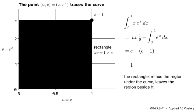
Let \(x\) run from 0 to 1 and follow the point \({(u, v) = (x, e^x)}\). It traces a curve from \({(0, 1)}\) to \({(1, e)}\). Draw the rectangle with corners \({(0, 0)}\) and \({(1, e)}\). The curve cuts it in two.
M04.7.2-F1
The curve traced by \({(u, v) = (x, e^x)}\) splits the rectangle \({uv = 1 \times e}\) into the region under it, \({\int v\,du = e - 1}\), and the region beside it, \({\int u\,dv}\), which is the integral we want. So \({\int_0^1 x\,e^x\,dx = e - (e - 1) = 1}\).
Name the two pieces. The region under the curve, between it and the \(u\)-axis, has area \({\int v\,du}\): here \(v\) is \(e^x\) and \(u\) moves from 0 to 1, so it is \({\int_0^1 e^x\,dx = e - 1}\), easy. The region beside the curve, between it and the \(v\)-axis, has area \({\int u\,dv}\): here \(u\) is \(x\) and \({dv = e^x\,dx}\), so it is \({\int_0^1 x\,e^x\,dx}\), the integral we want. Together they fill the rectangle, whose area is \({uv = 1 \times e}\). So
\[
\int_0^1 x\,e^x\,dx = e - (e - 1) = 1 .
\]
That is integration by parts: when one of the two areas is hard, find the other and subtract it from the rectangle.
Build it up
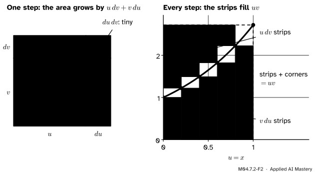
Step 1. One small step. The product rule (M04.3.3) says \({(uv)' = u'v + uv'}\). In the language of small changes: when \(u\) grows by \(du\) and \(v\) by \(dv\), the rectangle \(uv\) grows by a strip \({u\,dv}\) along the top, a strip \({v\,du}\) down the side, and a corner \({du\,dv}\) that is tiny by comparison.
M04.7.2-F2
The product rule as areas. Left: one step adds \({u\,dv + v\,du}\), plus a tiny corner. Right: step along the curve and the horizontal strips fill the region beside it while the vertical strips fill the region under it. As the steps shrink, the corners vanish.
Step 2. Add up all the steps. Integrate the product rule from \(a\) to \(b\). On the left, \(uv\) is an antiderivative of \({(uv)'}\), so part two of the fundamental theorem gives its total change:
In short, \({\int u\,dv = uv - \int v\,du}\). The term \({[uv]_a^b = u(b)v(b) - u(a)v(a)}\) is the boundary term.
Proof. Let \({w = uv}\). By the product rule, \({w' = u'v + uv'}\), and all three of \({w'}\), \({u'v}\) and \({uv'}\) are continuous, so they can be integrated. Integrate \({w' = u'v + uv'}\) from \(a\) to \(b\). Part two of the fundamental theorem turns the left side into \({w(b) - w(a)}\), and the sum rule for integrals (M04.5.3) splits the right side:
Subtracting \({\int_a^b u'v\,dx}\) from both sides gives the definite form. For the indefinite form: \(uv\) is an antiderivative of \({u'v + uv'}\), so \(uv\) minus an antiderivative of \({vu'}\) is an antiderivative of \({uv'}\). \(\blacksquare\)
Choosing \(u\). The formula is always true; what you choose decides whether it helps. Pick for \(u\) the factor that gets simpler when differentiated, and for \(dv\) a factor you can integrate without it getting worse. A power of \(x\) drops a degree when differentiated, and \({\ln x}\) turns into \({1/x}\); \({e^x}\), \({e^{-x}}\), sine and cosine stay the same size either way. A common rule of thumb lists the kinds of function in the order logarithms, inverse trigonometric functions, algebraic functions (powers), trigonometric functions, exponentials, and takes for \(u\) the one that comes first. It is a guide, not a law: when it fails, try the other choice.
Go deeper: does the constant in v matter?
Any antiderivative \(v\) of \({v'}\) will do. Replace \(v\) by \({v + K}\) for a constant \(K\). The term \(uv\) gains \({Ku}\), and \({\int v\,du}\) gains \({\int K\,du = Ku}\) (plus a constant). The two gains cancel in \({uv - \int v\,du}\), so the answer is unchanged. That is why the worked examples simply take the plainest antiderivative and leave the constant \(C\) to the very end.
Worked example
Example 1: \({\int x\,e^x\,dx}\). Differentiating \(x\) makes it simpler, and \(e^x\) integrates to itself. So take
\[
\begin{aligned}
u &= x, &\quad dv &= e^x\,dx, \\
du &= dx, &\quad v &= e^x .
\end{aligned}
\]
Check: the product rule gives \({((x - 1)e^x)' = e^x + (x - 1)e^x}\), which is \({x\,e^x}\). From 0 to 1 the answer is \({[(x - 1)e^x]_0^1 = 0 - (-1) = 1}\), the area of the anchor figure.
Example 2: \({\int \ln x\,dx}\). There is no visible product, but there is a hidden factor 1. Take \({u = \ln x}\), which gets simpler, and \({dv = dx}\):
\[
\begin{aligned}
\int \ln x\,dx &= x\ln x - \int x \cdot \frac{1}{x}\,dx \\
&= x\ln x - x + C .
\end{aligned}
\]
Check: \({(x\ln x - x)' = \ln x + 1 - 1 = \ln x}\). From 1 to \(e\) it gives \({(e - e) - (0 - 1) = 1}\). That is the grey region of the anchor figure again, seen from the side: the curve \({v = e^u}\) is the curve \({u = \ln v}\).
Example 3: \({\int x^2\,e^{-x}\,dx}\), two rounds. First check one antiderivative we need: \({(-e^{-x})' = e^{-x}}\), so \({-e^{-x}}\) is an antiderivative of \(e^{-x}\).
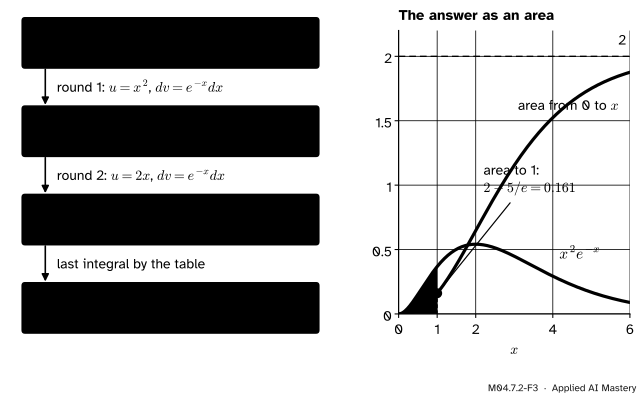
Round 1. Take \({u = x^2}\) and \({dv = e^{-x}\,dx}\), so \({du = 2x\,dx}\) and \({v = -e^{-x}}\):
Two rounds of parts, each lowering the power of \(x\) by one (left), and the result read as an area (right): the area under \({x^2 e^{-x}}\) from 0 to 1 is \({2 - 5/e \approx 0.161}\), and the area from 0 to \(x\) levels off at 2, a fact the next lesson makes precise.
From scratch first: a midpoint sum (M04.5.2) for each definite integral, beside the value found by parts, and a central difference (M04.2.4) to check each antiderivative.
import mathdef midpoint_sum(f, a, b, n=2000): dx = (b - a) / nreturnsum(f(a + (k +0.5) * dx) for k inrange(n)) * dxdef central(F, x, h=1e-5):return (F(x + h) - F(x - h)) / (2* h)cases = { # name: (integrand, antiderivative by parts, a, b)"x e^x": (lambda x: x * math.exp(x), lambda x: (x -1) * math.exp(x), 0, 1),"ln x": (math.log, lambda x: x * math.log(x) - x, 1, math.e),"x^2 e^(-x)": (lambda x: x**2* math.exp(-x), lambda x: -(x**2+2*x +2) * math.exp(-x), 0, 1),}by_parts, slope_gaps = {}, {}for name, (f, F, a, b) in cases.items(): by_parts[name] = F(b) - F(a) slope_gaps[name] =max(abs(central(F, x) - f(x)) for x in (1.2, 1.5, 2.0, 2.5))print(f"{name:11s} by parts {by_parts[name]:.6f} midpoint sum {midpoint_sum(f, a, b):.6f}"f" largest slope gap {slope_gaps[name]:.0e}")
x e^x       by parts 1.000000   midpoint sum 1.000000   largest slope gap 1e-09
ln x        by parts 1.000000   midpoint sum 1.000000   largest slope gap 9e-12
x^2 e^(-x)  by parts 0.160603   midpoint sum 0.160603   largest slope gap 7e-12
All three agree. The boundary term is not optional: drop it from Example 1 and the “answer” is \({-\int_0^1 e^x\,dx}\), a negative number for a positive integrand.
with_boundary = (1* math.e -0*1) - (math.e -1) # [x e^x] from 0 to 1, minus the integral of e^xwithout_boundary =-(math.e -1)print(f"with the boundary term {with_boundary:.4f}, without it {without_boundary:.4f}")
with the boundary term 1.0000, without it -1.7183
The library confirms all three with scipy.integrate.quad, which returns the value and an estimate of its error.
from scipy import integratefor name, (f, F, a, b) in cases.items(): value, error = integrate.quad(f, a, b)print(f"{name:11s} quad {value:.10f} error estimate {error:.0e}")
This module’s interactive, the substitution viewer, lives in lesson M04.7.1. Integration by parts has its own picture in the anchor figure above. To see that \({\int u\,dv}\) really is the area beside the curve, change the variable in it: along the curve \({v = e^u}\), the region beside it is the region under \({u = \ln v}\) for \(v\) from 1 to \(e\), which is Example 2.
Pitfalls
M04.7.2-F4
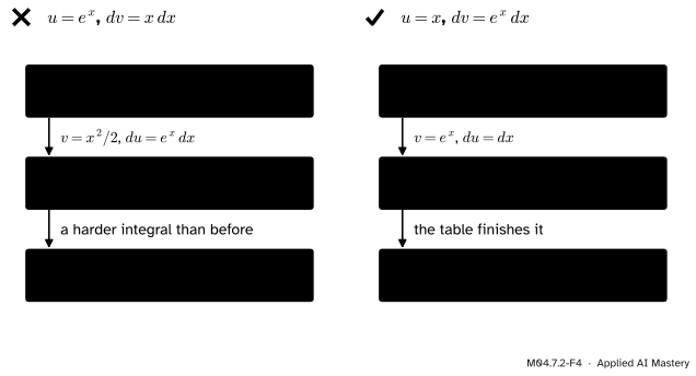
Wrong beside right for \({\int x\,e^x\,dx}\). Choosing \({u = e^x}\) (left) raises the power of \(x\) and leaves a harder integral. Choosing \({u = x}\) (right) lowers it, and the table finishes the job.
“Any split into \(u\) and \(dv\) will do.”
Every split gives a true equation, but only some give an easier integral. With \({u = e^x}\) and \({dv = x\,dx}\), the new integral is \({\int \frac{x^2}{2} e^x\,dx}\), worse than the one you started with, and a second round would make it worse again. If the power of \(x\) goes up, swap the roles.
“In a definite integral, only the last integral needs limits.”
The boundary term \({[uv]_a^b}\) is part of the answer. For \({\int_0^1 x\,e^x\,dx}\) it is \({[x\,e^x]_0^1 = e}\), and without it the result is \({-(e - 1) \approx -1.718}\), negative although the integrand is positive on the whole interval. A sign check like that catches the slip.
“\(v\) is the integral of \(dv\), so the sign takes care of itself.”
The antiderivative of \(e^{-x}\) is \({-e^{-x}}\), and in Example 3 that minus sign appears in both rounds. Losing it once gives \({-(x^2 - 2x + 2)\,e^{-x}}\) or a similar wrong answer. Differentiating the result, by hand or with the central difference above, finds the slip in seconds.
Frontier note: integration by parts inside score matching
Many models give a density only up to a constant that cannot be computed. Hyvärinen (2005) fits such a model by matching its score, the slope of the log-density, \({\psi = (\ln p)'}\), to the slope of the log-density of the data. The squared gap between the two seems to need the data’s own score, which is unknown. His Theorem 1 removes it with “a simple trick of partial integration”: in one dimension, the troublesome term is \({\int \psi(x)\,p_{\text{data}}'(x)\,dx}\), and parts turns it into \({-\int \psi'(x)\,p_{\text{data}}(x)\,dx}\), an average over the data that needs only the model. The boundary term vanishes because, by assumption, \({p_{\text{data}}\,\psi}\) goes to zero far out, an integral over an infinite range of the kind the next lesson defines. Score-based generative models (Song and Ermon, 2019) learn with score matching the slopes from which they then draw samples.
Check yourself
Recall
1. State the integration-by-parts formula in its short form.
Show answer
\({\int u\,dv = uv - \int v\,du}\).
2. Which rule of differentiation is it the reverse of?
Show answer
The product rule, \({(uv)' = u'v + uv'}\), integrated and rearranged.
3. In \({\int x\,e^x\,dx}\), which choice of \(u\) works, and what goes wrong with the other?
Show answer
\({u = x}\), \({dv = e^x\,dx}\) works: the new integral is \({\int e^x\,dx}\). With \({u = e^x}\) and \({dv = x\,dx}\) the new integral is \({\int \frac{x^2}{2}e^x\,dx}\), harder than the original.
4. How do you integrate \({\ln x}\) by parts, and what is the result?
Show answer
Take \({u = \ln x}\) and \({dv = dx}\), so \({du = dx/x}\) and \({v = x}\). The result is \({x\ln x - x + C}\).
5. What is the boundary term of the definite form, and what is it for \({\int_0^1 x\,e^x\,dx}\)?
Show answer
\({[uv]_a^b = u(b)v(b) - u(a)v(a)}\). For this integral it is \({[x\,e^x]_0^1 = e - 0 = e}\).
Exercises
1.★ Find \({\int x\,e^{-x}\,dx}\), and then \({\int_0^1 x\,e^{-x}\,dx}\).
Show solution
Take \({u = x}\), \({dv = e^{-x}\,dx}\), so \({du = dx}\) and \({v = -e^{-x}}\):
From 0 to 1: \({-16/e - (-6)}\), which is \({6 - 16/e \approx 0.1139}\). The constants 1, 2, 6 left at the ends of these formulas are \({1!}\), \({2!}\), \({3!}\); the next lesson shows why that matters.
Summary card
Integration by parts trades \({\int u\,dv}\) for \({\int v\,du}\): the rectangle \(uv\) minus the other piece.
M04.7.2-F1
Rectangle minus one region leaves the other.
Formula.\({\int u\,dv = uv - \int v\,du}\), from the product rule.
Definite form. Keep the boundary term \({[uv]_a^b}\).
Choose \(u\) to get simpler when differentiated: powers of \(x\), \({\ln x}\).
Results.\({(x - 1)e^x}\), \({x\ln x - x}\) and \({-(x^2 + 2x + 2)e^{-x}}\), each plus \(C\).
Sources and next steps
Sources. Each was opened and checked against this lesson on 12 November 2026.
Gilbert Strang and Edwin Herman, Calculus Volume 2 (OpenStax), Section 3.1, Integration by parts: the derivation from the product rule, the formula (Equation 3.1, Theorem 3.1) and its definite form (Equation 3.2), the rule of thumb for choosing \(u\) (the order logarithmic, inverse trigonometric, algebraic, trigonometric, exponential, with the remark that it can fail), and Example 3.3, which needs two rounds.
Matthew Boelkins, Active Calculus (single variable), Section 5.4, Integration by parts: the derivation from the product rule (Subsection 5.4.2), the advice to choose \(u\) and \(dv\) so that the new integral is no harder than the old, Example 5.4.2 with two rounds, and definite integrals with the boundary term (Subsection 5.4.5).
David Jerison, MIT OpenCourseWare 18.01SC, Session 76, Integration by parts: the method for a product of an easy and a hard function, applied more than once when needed, with a lecture clip on the integral of the natural logarithm.
Aapo Hyvärinen, Estimation of non-normalized statistical models by score matching, Journal of Machine Learning Research 6, 695 to 709 (2005), Section 2: the score-matching objective and Theorem 1, proved by partial integration, with the condition that the density times the model score goes to zero far out.