Cut an interval into equal strips, take a height in each, and add height times width: a Riemann sum. For x squared on [0, 1] the right sums have a closed form that tends to exactly 1/3, and that limit is the definite integral. Compute the sums by hand, by a loop and with NumPy.
Compute left, right and midpoint sums by hand for a function on an interval cut into equal strips.
Derive the closed form (n + 1)(2n + 1)/(6n^2) of the right sum of x^2 on [0, 1], using the sum of the first n squares proved by induction, and find its limit 1/3.
State the definition of the definite integral as a limit of Riemann sums, and name each part of its notation.
Write a riemann_sum function with a loop, then vectorise it with NumPy.
In review. The maths and code on this page are checked by automated tests on every change, but an independent reader has not signed it off yet. Spot a mistake or a confusing step? Tell us.
The question
The region under the curve \({y = x^2}\), from \({x = 0}\) to \({x = 1}\), is not a rectangle, a triangle or a circle, so no school formula gives its area. Rectangles can come as close to it as we like, but every finite set of them is a little off. How can rectangles give an exact number? The answer, a limit of sums, is the definite integral. In machine learning it is the quantity behind every probability and every expected value of a continuous variable, and behind the area under an ROC curve.
From the last lesson
1. For a speed that only rises, which of the left and right sums is too small?
Show answer
The left sum, because each of its rectangles uses the lowest speed on its slice.
2. What is the gap between the right and left sums with \(n\) equal slices from \(a\) to \(b\)?
Show answer
\({(v(b) - v(a))\,\Delta t}\) with \({\Delta t = (b - a)/n}\): the rise in height times one slice width.
Intuition
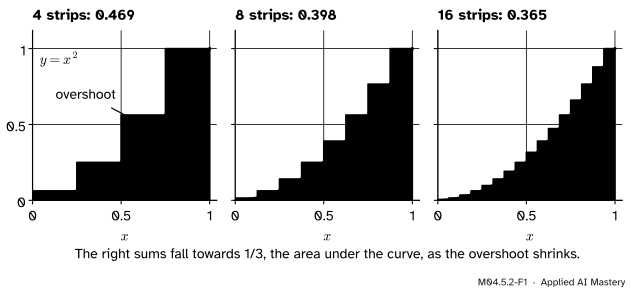
Lesson M04.5.1 trapped a distance between two sums of rectangles. The same rectangles work for any curve. Cut the interval into strips, stand a rectangle on each strip, and add the rectangles’ areas. The thinner the strips, the less each rectangle overshoots or falls short of the curve.
M04.5.2-F1
Riemann sums refining. Each time the strips halve, the overshoot shrinks and the sum of the rectangles falls closer to the area under the curve, 1/3.
The sums 0.469, 0.398 and 0.365 are settling down. The number they settle on is the area, and this lesson proves that it is exactly 1/3.
Build it up
Step 1. Strips. Cut the interval from \(a\) to \(b\) into \(n\) strips of equal width
\[
\cparam{\Delta x} = \frac{b - a}{n} .
\]
The cut points are \({x_k = a + k\,\Delta x}\) for \({k = 0, 1, \dots, n}\), and strip \(k\) runs from \(x_{k-1}\) to \(x_k\), for \(k\) from 1 to \(n\).
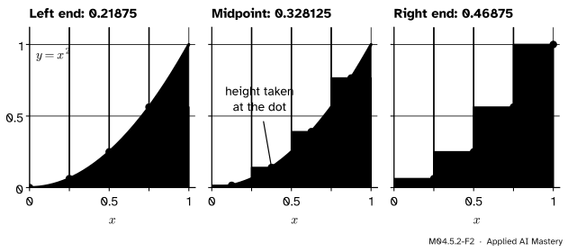
Step 2. A height for each strip. Choose a sample point\(x_k^*\) somewhere in strip \(k\) and use \({f(x_k^*)}\) as the rectangle’s height. The three common choices are the left end, the right end and the middle of the strip.
M04.5.2-F2
One set of strips, three choices of height. The dot in each strip is its sample point. The midpoint rectangles cross the curve, so their overshoots and shortfalls nearly cancel.
Step 3. The Riemann sum. Add height times width over all the strips:
\[
\sum_{k=1}^{n} f(x_k^*)\,\Delta x .
\]
Any sum of this form is a Riemann sum. The left, right and midpoint sums take \({x_k^* = x_{k-1}}\), \({x_k^* = x_k}\) and the middle of the strip. We write them \({\text{Left}(n)}\), \({\text{Right}(n)}\) and \({\text{Mid}(n)}\).
Step 4. Let the strips shrink. For \({f(x) = x^2}\) the curve rises from 0 to 1, so by lesson M04.5.1 the true area lies between the left and right sums, whose gap is \({(f(1) - f(0))\,\Delta x = 1/n}\). To pin the area down we need the value those sums approach as \(n\) grows. For the right sum we can find it exactly.
The formal statement
The right sum in closed form. On \({[0, 1]}\) the strip width is \({\Delta x = 1/n}\) and the right ends are \({x_k = k/n}\). So
The factor \({1/n^3}\) is the same in every term, so it comes outside the sigma (the constant-factor rule of M01.7.2). What is left is the sum of the first \(n\) squares.
The sum of the first \(n\) squares. For every whole number \({n \ge 1}\),
Proof by induction (M01.6.4). At \({n = 1}\) the left side is 1 and the right side is \({1 \times 2 \times 3 / 6 = 1}\). Now suppose the formula holds for some \(n\). Adding the next square,
The third line takes out the common factor \({n + 1}\), the fourth multiplies out the bracket, and the last factorises \({2n^2 + 7n + 6}\) as \({(n + 2)(2n + 3)}\). Since \({(n + 1) + 1 = n + 2}\) and \({2(n + 1) + 1 = 2n + 3}\), the result is the formula with \({n + 1}\) in place of \(n\). So the formula holds for every \(n\).
The closed form and its limit. Put the formula into the right sum. One factor \(n\) cancels:
The left sums agree. The gap is \({1/n}\), so \({\text{Left}(n) = \text{Right}(n) - 1/n}\), which also tends to 1/3. Every midpoint height lies between the left and right heights of its strip, so \({\text{Mid}(n)}\) is squeezed between the two and tends to 1/3 as well (the squeeze theorem of M04.1.2).
NoteDefinition: the definite integral
For a function \(f\) on \({[a, b]}\), cut into \(n\) equal strips of width \({\Delta x = (b - a)/n}\) with a sample point \(x_k^*\) in strip \(k\), the definite integral of \(f\) from \(a\) to \(b\) is
when this limit exists and is the same for every choice of sample points.
M04.5.2-F5
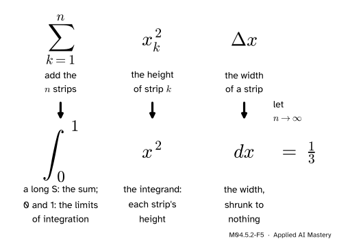
Each part of the notation comes from a part of the sum. The sigma becomes the integral sign, the height \(x_k^2\) becomes the integrand \(x^2\), and the width \({\Delta x}\) becomes \(dx\).
The parts have names. The function \(f\) is the integrand, \(a\) and \(b\) are the limits of integration, and \(x\) is the variable of integration. Like the index of a sigma, \(x\) is a dummy: \({\int_0^1 x^2\,dx}\) and \({\int_0^1 t^2\,dt}\) are the same number. We have proved
\[
\int_0^1 x^2\,dx = \frac{1}{3} .
\]
When does the limit exist? For every continuous function on \({[a, b]}\) it does, and every choice of sample points gives the same limit. This theorem is stated here without proof; its proof uses a property of the real numbers that belongs to analysis. A function with a few jumps, such as a step, has an integral too (lesson M04.6.2 uses one), but every function in this module is continuous where we integrate it.
Go deeper: why every choice of sample point gives the same limit, for a rising function
Suppose \(f\) never falls on \({[a, b]}\). In strip \(k\) any sample point \(x_k^*\) lies between \(x_{k-1}\) and \(x_k\), so \({f(x_{k-1}) \le f(x_k^*) \le f(x_k)}\). Multiply by \({\Delta x > 0}\) and add over the strips:
The gap between the outer sums is \({(f(b) - f(a))\,\Delta x}\) (M04.5.1, Result 2), which tends to 0. So once either outer sum is known to tend to a number, every Riemann sum tends to the same number, by the squeeze theorem. For \({x^2}\) on \({[0, 1]}\) we found that number exactly: whatever sample points you choose, the sums tend to 1/3. A function that never rises works the same way, with the inequalities turned round.
Worked example
Find the left, right and midpoint sums of \({f(x) = x^2}\) on \({[0, 1]}\) with four strips.
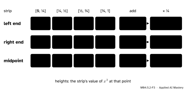
Here \({\Delta x = 1/4}\) and the cut points are 0, 1/4, 1/2, 3/4 and 1, where the heights are 0, 1/16, 4/16, 9/16 and 16/16. The midpoints are 1/8, 3/8, 5/8 and 7/8, where the heights are 1/64, 9/64, 25/64 and 49/64.
M04.5.2-F3
The hand computation, one row per rule: four heights, their total, and the total times the strip width, which gives the sum.
Each sum is the total of its heights times \({\Delta x = 1/4}\):
As decimals these are 0.21875, 0.46875 and 0.328125. The right sum’s numerator, \({1 + 4 + 9 + 16}\), is the sum of the first four squares, 30, and the closed form agrees: with \({n = 4}\) it gives \({(5 \times 9)/(6 \times 16)}\), which is \({45/96 = 0.46875}\).
Compare with the exact area 1/3, about 0.33333. The left sum is short by 0.115 and the right sum over by 0.135, but the midpoint sum is short by only 0.0052, more than twenty times closer. Its rectangles cross the curve, so in each strip the part that overshoots nearly cancels the part that falls short.
Code
One function covers all three rules. The sample point sits a fraction shift of the way across its strip: 0 for the left end, 0.5 for the middle and 1 for the right end.
def riemann_sum(f, a, b, n, rule="mid"):"""A Riemann sum of f over [a, b] with n equal strips.""" dx = (b - a) / n shift = {"left": 0.0, "mid": 0.5, "right": 1.0}[rule] total =0.0for k inrange(n): # strip k + 1 runs from a + k dx to a + (k + 1) dx x = a + (k + shift) * dx # its sample point total = total + f(x) * dx # height times widthreturn totaldef f(x):return x **2for rule in ["left", "right", "mid"]:print(f"{rule:5s} sum, 4 strips: {riemann_sum(f, 0, 1, 4, rule)}")
left  sum, 4 strips: 0.21875
right sum, 4 strips: 0.46875
mid   sum, 4 strips: 0.328125
Now check the closed form against the loop, and watch the error shrink.
for n in [4, 16, 64, 256, 1024]: loop = riemann_sum(f, 0, 1, n, "right") closed = (n +1) * (2* n +1) / (6* n **2)print(f"n = {n:4d}: loop {loop:.6f}, closed form {closed:.6f}, error {loop -1/3:.6f}")
n =    4: loop 0.468750, closed form 0.468750, error 0.135417
n =   16: loop 0.365234, closed form 0.365234, error 0.031901
n =   64: loop 0.341187, closed form 0.341187, error 0.007853
n =  256: loop 0.335289, closed form 0.335289, error 0.001956
n = 1024: loop 0.333822, closed form 0.333822, error 0.000488
The error is \({1/(2n) + 1/(6n^2)}\), as derived. Each row has four times as many strips as the one before and about a quarter of its error, so doubling \(n\) about halves the error. A loop over a million strips is slow in plain Python. NumPy makes all the sample points at once with numpy.arange and adds the heights with numpy.sum.
import numpy as npdef riemann_sum_np(f, a, b, n, rule="mid"):"""The same sum, with every sample point made at once.""" dx = (b - a) / n shift = {"left": 0.0, "mid": 0.5, "right": 1.0}[rule] x = a + (np.arange(n) + shift) * dx # all n sample pointsreturn np.sum(f(x)) * dxprint("NumPy, 4 strips:", riemann_sum_np(f, 0, 1, 4, "mid"))print(f"NumPy, a million strips: {riemann_sum_np(f, 0, 1, 1_000_000, 'mid'):.10f}")
NumPy, 4 strips: 0.328125
NumPy, a million strips: 0.3333333333
With a million strips the midpoint sum matches 1/3 to at least nine decimal places. The last few digits depend on rounding inside the computer, so the check allows for that.
Explore
M04.5-X1
Riemann refiner
Choose \({y = x^2}\) and the right rule, then press Double the strips a few times: the sum falls towards 1/3 and the error about halves each time. Switch to the midpoint rule and the error is far smaller and falls by about four. Try the cart’s speed and the bell curve, and the cart run on to 5 s, whose curve dips below the axis.
Pitfalls
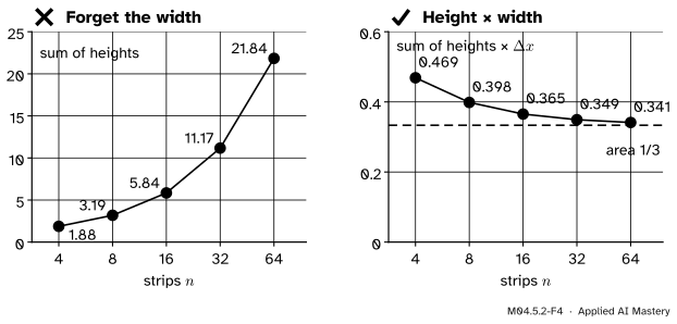
M04.5.2-F4
Wrong beside right. Without the widths the total grows without limit, roughly like \({n/3}\). With them it settles on the area.
“A Riemann sum adds up the heights.”
It adds up heights times widths. Leave out \({\Delta x}\) and the total grows with the number of strips: for \({x^2}\) the right-end heights alone add to 1.875 with 4 strips and 21.8 with 64. In code this is the missing * dx, a common bug when an expected value or an area is computed from samples.
“The midpoint sum is the average of the left and right sums.”
The average of 0.21875 and 0.46875 is 0.34375, but the midpoint sum is 0.328125. The midpoint rule takes the height of the curve at the middle of each strip, while the average of the two sums averages the heights at the ends. For a curve that bends upwards, like \({x^2}\), the middle height is lower. The average of the two sums is a rule of its own, the trapezoid rule of lesson M04.5.4.
“With enough strips, the sum is the integral.”
A finite sum is in general only an approximation. For \({x^2}\) the right sum is \({1/3 + 1/(2n) + 1/(6n^2)}\), which is above 1/3 for every \(n\). The integral is the limit, the one number that all the sums approach.
Check yourself
Recall
1. What is the strip width for \(n\) equal strips on \({[a, b]}\)?
Show answer
\({\Delta x = (b - a)/n}\).
2. Where does the midpoint rule take each strip’s height?
Show answer
At the middle of the strip, \({(x_{k-1} + x_k)/2}\), where the height is \({f\big((x_{k-1} + x_k)/2\big)}\).
3. What is \({1^2 + 2^2 + \dots + n^2}\) in closed form, and how was it proved?
Show answer
\({n(n + 1)(2n + 1)/6}\), proved by induction: true for \({n = 1}\), and true for \({n + 1}\) whenever it is true for \(n\).
4. Write the definition of \({\int_a^b f(x)\,dx}\).
As decimals these are 0.125, 0.625 and 0.3125. The closed form gives \({(3 \times 5)/(6 \times 4)}\), which is \({15/24 = 5/8}\), as it should.
2.★★ Find the smallest \(n\) for which the right sum of \({x^2}\) on \({[0, 1]}\) is within 0.001 of 1/3.
Show solution
The error is \({1/(2n) + 1/(6n^2)}\), and it is more than \({1/(2n)}\). So we need \({1/(2n) < 0.001}\), that is \({n > 500}\). At \({n = 500}\) the error is \({0.001 + 1/1\,500\,000}\), just too big. At \({n = 501}\) it is
The last fraction is the right sum on \({[0, 1]}\), which tends to 1/3. So the right sums tend to \({b^3/3}\). The function rises on \({[0, b]}\), so by the squeeze argument in the formal statement every Riemann sum has the same limit. For \({b = 2}\) the area is \({8/3}\).
Summary card
The definite integral is the limit of Riemann sums as the strips shrink.
M04.5.2-F1
More strips, less overshoot.
Riemann sum. Add \({f(x_k^*)\,\Delta x}\) over the strips, where \({\Delta x = (b - a)/n}\).
Right sums of \({x^2}\). They equal \({\tfrac13 + \tfrac{1}{2n} + \tfrac{1}{6n^2}}\), which tends to 1/3.
The integral.\({\int_0^1 x^2\,dx = 1/3}\), and \({\int_0^b x^2\,dx = b^3/3}\).
Sources and next steps
Sources. Each was opened and checked against this lesson on 12 November 2026.
Gilbert Strang and Edwin Herman, Calculus Volume 1 (OpenStax), Section 5.1, Approximating Areas, which gives the sum of the first \(n\) squares under “Rule: Sums and Powers of Integers” and defines a Riemann sum with any sample point in each subinterval; and Section 5.2, The Definite Integral, which defines the integral as the limit of Riemann sums (equation 5.8), names the integrand, the limits of integration and the variable of integration, a dummy variable, and states without proof that continuous functions are integrable (Theorem 5.1), adding that a function with finitely many jumps is integrable too.
David Jerison, MIT OpenCourseWare 18.01SC, Session 46: Riemann Sums, and its lecture notes, which set out the procedure used here: divide \({[a, b]}\) into \(n\) equal pieces, pick any point in each, add height times width, and let \(n\) grow.
Matthew Boelkins, Active Calculus, Section 4.2, “Riemann sums”, which introduces the left, right and middle sums, written \(L_n\), \(R_n\) and \(M_n\). This course writes them \({\text{Left}(n)}\), \({\text{Right}(n)}\) and \({\text{Mid}(n)}\) because \(L\) is the loss and \(T_n\) a Taylor polynomial.