At a steady speed, distance is speed times time, the area of a rectangle under the speed graph. When the speed changes, cut time into thin slices, treat each as steady and add the rectangles. The left and right sums trap the true distance, and the gap between them shrinks with the slices.
Compute a distance at constant speed as the area of a rectangle under the speed graph, and give the units of an area under any rate curve.
Approximate the distance covered at a changing speed by a left sum and a right sum of thin rectangles, and write both in sigma notation.
Explain why, for a speed that only rises, the left sum is too small and the right sum too large, and derive that the gap between them is the rise in speed times the width of one slice.
Code both sums with a plain loop and show the gap closing as the slices get thinner.
In review. The maths and code on this page are checked by automated tests on every change, but an independent reader has not signed it off yet. Spot a mistake or a confusing step? Tell us.
The question
A cart’s speedometer is read once a second: 0, 3, 4, 3 and 0 metres per second. How far did the cart go? If its speed never changed, distance would be speed times time, but the speed changes all the time. The same question comes up whenever a system logs a rate instead of a total. A training run reports examples per second and a power meter reports watts, yet what you want to know is the number of examples seen and the energy used. Those totals have to be built from the rates.
Intuition
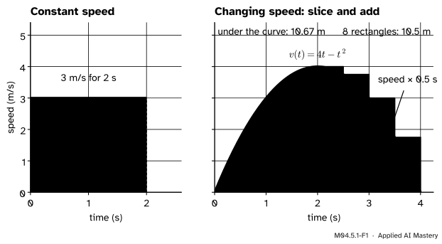
At a constant speed, distance is speed times time. On a graph of speed against time a constant speed is a flat line, and the distance is the area of the rectangle under it: its height is the speed, its width is the time, and height times width is speed times time.
M04.5.1-F1
Distance is the area under the speed graph. Left: at a constant speed that area is a rectangle. Right: when the speed changes, cut time into slices, treat the speed as constant on each, and add the rectangles. Their total, 10.5 m, is close to the area under the curve, 10.67 m.
When the speed changes, no single rectangle fits under the graph. But over a short enough slice of time the speed hardly changes, so on that slice the rectangle rule nearly works. Cut the trip into thin slices, give each slice a rectangle, and add them up. The thinner the slices, the closer the total comes to the area under the speed curve, and that area is the distance.
Build it up
The running trip of this course is a cart, an invented example, whose speed is \({v(t) = 4t - t^2}\) metres per second for \(t\) from 0 to 4 seconds. Its speed rises from 0 to a top speed of 4 m/s at \({t = 2}\) and falls back to 0 at \({t = 4}\). Sampled once a second, its speeds are 0, 3, 4, 3 and 0. Start with the first two seconds, while the cart speeds up.
Step 1. Constant speed. A cart that holds 3 m/s for 2 s goes \({3 \times 2 = 6}\) m: the area of the rectangle in the left panel of the figure above.
Step 2. A speed that jumps. A cart that does 3 m/s for one second and then 4 m/s for one second goes \({3 \times 1 + 4 \times 1 = 7}\) m: two rectangles side by side. Whenever a speed changes only in jumps, the distance is a sum of rectangles.
Step 3. A speed that changes smoothly. Our cart’s speed changes at every instant, so pretend that it jumps. Cut the two seconds into two slices of one second, and on each slice use one speed for the whole slice: the speed at the slice’s start, or the speed at its end.
Step 4. Two answers that trap the truth. With the starting speeds, 0 and 3, the rectangles add to \({0 \times 1 + 3 \times 1 = 3}\) m. With the ending speeds, 3 and 4, they add to \({3 \times 1 + 4 \times 1 = 7}\) m. The cart speeds up all the time, so during each slice it goes at least its starting speed and at most its ending speed. The true distance \(d\) lies between: \({3 \le d \le 7}\).
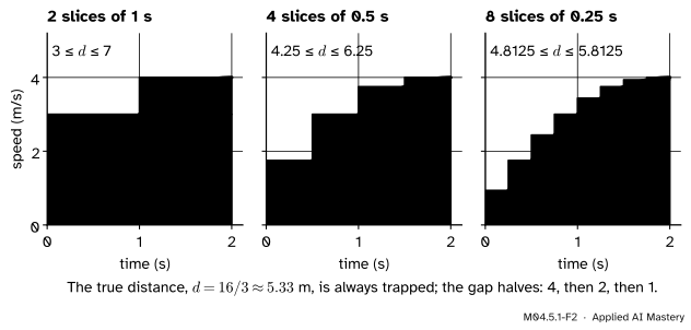
Step 5. Thinner slices. Halve the slices to half a second. The speeds at 0, 0.5, 1, 1.5 and 2 s are 0, 1.75, 3, 3.75 and 4. The starting speeds give
The trap has shrunk from a width of 4 m to a width of 2 m.
M04.5.1-F2
Each time the slices halve, the left sum rises, the right sum falls, and the gap between them halves. The true distance stays trapped between the two.
Halve the slices again and the gap halves again, to 1 m. The true distance, 16/3 or about 5.33 m (the worked example finds it), sits inside every trap.
The formal statement
NoteDefinition: left and right sums
Cut the time from \(a\) to \(b\) into \(n\) slices of equal width
\[
\cparam{\Delta t} = \frac{b - a}{n},
\]
with cut points \({t_k = a + k\,\Delta t}\) for \({k = 0, 1, \dots, n}\). The left sum takes each slice’s height at its start and the right sum at its end:
\[
\begin{aligned}
\text{Left}(n) &= \sum_{k=0}^{n-1} v(t_k)\,\Delta t , \\
\text{Right}(n) &= \sum_{k=1}^{n} v(t_k)\,\Delta t .
\end{aligned}
\]
Both sums run over the same \(n\) slices. The left sum uses the cut points \(t_0\) to \(t_{n-1}\) and the right sum uses \(t_1\) to \(t_n\). Each term \({v(t_k)\,\Delta t}\) is one rectangle: a speed times a time, which is a distance. The sigma is the loop of M01.7: start at 0 and add one term per slice.
Units. An area under a rate curve carries the units of the rate times the units of the input: here (m/s) × s = m. A graph of examples per second against seconds has areas measured in examples, and a graph of watts against seconds has areas measured in joules.
Result 1: the trap. If \(v\) never falls between \(a\) and \(b\), then for every \(n\)
where \(d\) is the distance travelled from \(a\) to \(b\). If \(v\) never rises, the inequalities turn round.
Why. On the slice from \(t_{k-1}\) to \(t_k\) the speed is at least \({v(t_{k-1})}\) and at most \({v(t_k)}\). Moving for a time \(\Delta t\) at such speeds, the cart covers at least \({v(t_{k-1})\,\Delta t}\) and at most \({v(t_k)\,\Delta t}\). Add these over the \(n\) slices: the distances covered on the slices add up to \(d\), the lower bounds add up to the left sum, and the upper bounds add up to the right sum.
Result 2: the gap. For any \(v\), rising, falling or neither,
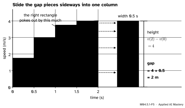
Result 2 as a picture. Each right rectangle pokes out above its left neighbour by a thin piece. Slid sideways, the pieces stack exactly into one column, as tall as the whole rise in speed and one slice wide.
For the cart’s first two seconds, \({v(2) - v(0) = 4}\) and \({b - a = 2}\), so the gap is \(8/n\) metres: 4, 2 and 1 for \({n = 2, 4, 8}\). The speed only rises there, so by Result 1 the distance is trapped in a window \(8/n\) wide. That window shrinks to nothing as \(n\) grows, so both sums close in on \(d\).
Go deeper: the trap, proved from the mean value theorem
The step “moving at a speed of at most \(M\) for a time \(\Delta t\) covers at most \(M\,\Delta t\)” can be proved with the mean value theorem of M04.4.1.
Let \({s(t)}\) be the cart’s position, so that \({s'(t) = v(t)}\), and suppose \({v(t) \le M}\) on the slice from \(t_{k-1}\) to \(t_k\). The function \({h(t) = s(t) - M t}\) has derivative \({h'(t) = v(t) - M \le 0}\). By the mean value theorem there is a time \(c\) in the slice with
Move the \(M\) terms to the right and use \({t_k - t_{k-1} = \Delta t}\):
\[
s(t_k) - s(t_{k-1}) \le M\,\Delta t .
\]
If instead \({v(t) \ge m}\), the function \({s(t) - m t}\) never falls, and the same steps give \({s(t_k) - s(t_{k-1}) \ge m\,\Delta t}\). For a rising speed take \({m = v(t_{k-1})}\) and \({M = v(t_k)}\), then add over the slices. The middle positions cancel in pairs, as in Result 2, and the slice distances add up to \({s(b) - s(a) = d}\).
Worked example
How far does the cart go in its first two seconds? Use the table of speeds first, then check the answer against the cart’s position.
M04.5.1-F3
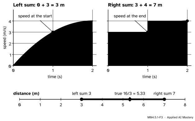
The trace of the two sums with one-second slices. Each rectangle is a speed from the table times one second. The true distance, 16/3 m, lies between the two totals.
One-second slices. Here \({\Delta t = 1}\) and the cut points are 0, 1 and 2 s, where the table gives 0, 3 and 4 m/s. The left sum uses the first two speeds and the right sum the last two:
and the right sum is \({0.5 \times (1.75 + 3 + 3.75 + 4) = 6.25}\). Result 2 predicts the gap \({(4 - 0) \times 0.5 = 2}\), and indeed \({6.25 - 4.25 = 2}\).
The check. The cart’s position is \({s(t) = 2t^2 - t^3/3}\) metres, whose derivative is the speed \(v(t)\) (M04.3.1 found it). The distance covered in the first two seconds is the change in position:
Both traps hold it: \({3 \le 5.33 \le 7}\) and \({4.25 \le 5.33 \le 6.25}\). The left sum is short because each rectangle uses the lowest speed on its slice; the right sum is long because each uses the highest.
Code
Each sum is a loop that keeps a running total, exactly as the sigma says. The functions take the speed as an argument f, so they work for any rate.
def v(t):"""The running trip's speed, in metres per second."""return4* t - t **2def left_sum(f, a, b, n):"""n rectangles, each as tall as f at the start of its slice.""" dt = (b - a) / n total =0.0for k inrange(n): # k = 0, 1, ..., n - 1 total = total + f(a + k * dt) * dtreturn totaldef right_sum(f, a, b, n):"""n rectangles, each as tall as f at the end of its slice.""" dt = (b - a) / n total =0.0for k inrange(1, n +1): # k = 1, 2, ..., n total = total + f(a + k * dt) * dtreturn totald =2*2**2-2**3/3# s(2) - s(0), the true distanceprint("true distance:", round(d, 4))for n in [2, 4, 8, 64, 1024]: lo, hi = left_sum(v, 0, 2, n), right_sum(v, 0, 2, n)print(f"n = {n:5d}: {lo:.4f} <= d <= {hi:.4f} gap {hi - lo:.4f}")
true distance: 5.3333
n =     2:  3.0000 <= d <= 7.0000   gap 4.0000
n =     4:  4.2500 <= d <= 6.2500   gap 2.0000
n =     8:  4.8125 <= d <= 5.8125   gap 1.0000
n =    64:  5.2705 <= d <= 5.3955   gap 0.1250
n =  1024:  5.3294 <= d <= 5.3372   gap 0.0078
The gap is \({8/n}\) every time, as Result 2 says, and the true distance never leaves the trap. With 1024 slices the two sums agree to within 0.008 m.
Real data often comes as a table rather than a formula. The same two sums work on a list of readings taken \({\Delta t}\) apart: the left sum uses every reading but the last, the right sum every reading but the first.
speeds = [0, 3, 4, 3, 0] # the table: t = 0, 1, 2, 3, 4 secondsdt =1.0left =sum(speeds[:-1]) * dt # readings at the starts of the slicesright =sum(speeds[1:]) * dt # readings at the ends of the slicesprint("whole trip, left sum:", left, " right sum:", right)print("true distance s(4) - s(0):", round(2*4**2-4**3/3, 4))
whole trip, left sum: 10.0   right sum: 10.0
true distance s(4) - s(0): 10.6667
Over the whole trip both sums give 10 m, yet the true distance is 32/3, about 10.67 m. The pitfalls below explain why agreement is not proof.
Explore
This module’s interactive, the Riemann refiner, lives in lesson M04.5.2. Choose the cart’s speed and the left or the right rule, then slide the number of strips: the rectangles redraw and the read-out shows the sum, the true area and the error shrinking.
Pitfalls
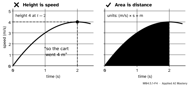
M04.5.1-F4
Wrong beside right. The height of the speed graph at a moment is a speed, 4 m/s. The distance covered up to that moment is the area under the graph, 16/3 m.
“The graph is at 4 when t is 2, so the cart has gone 4 metres.”
The height of a speed graph is a speed, in metres per second. The distance up to \({t = 2}\) is the area under the graph up to \({t = 2}\), which is 16/3 m. The same mix-up happens with any rate: the height of a throughput curve says how fast examples arrive, while the area says how many arrived.
“The left and right sums agree, so they must be exact.”
Over the whole trip both are 10 m, but the distance is 32/3 m. Result 2 says why they agree: their gap is \({(v(4) - v(0))\,\Delta t}\), and the speed is 0 at both ends. Agreeing is not the same as trapping. The trap of Result 1 needs a speed that only rises or only falls, and this one rises and then falls. Split the trip at \({t = 2}\), where the speed turns round, and trap each half separately; with one-second slices that gives \({6 \le d \le 14}\).
“An area under a graph is in square units.”
Only when both axes are lengths. An area under a rate curve has the units of the rate times the units of the input: (m/s) × s = m, and watts × seconds = joules.
“The right sum is the same loop as the left sum.”
The right sum must use the cut points \({t_1}\) to \({t_n}\), so its loop is range(1, n + 1). Writing range(n) in both functions silently computes the left sum twice.
Check yourself
Recall
1. A cart holds 5 m/s for 3 s. How far does it go, and what shape is that distance on a speed graph?
Show answer
15 m: the area of the rectangle under the flat speed line, 5 high and 3 wide.
2. A graph shows power in watts against time in seconds. What are the units of an area under it?
Show answer
Watts times seconds, which is joules: an amount of energy.
3. Write the left sum with \(n\) equal slices from \(a\) to \(b\) in sigma notation.
Show answer
\[
\text{Left}(n) = \sum_{k=0}^{n-1} v(t_k)\,\Delta t ,
\]
with \({\Delta t = (b - a)/n}\) and \({t_k = a + k\,\Delta t}\).
4. For a speed that only rises, which sum is too small and which too large?
Show answer
The left sum is too small, because each rectangle uses the lowest speed on its slice. The right sum is too large, because each uses the highest.
5. What is the gap between the right and left sums for the cart’s first two seconds with \(n\) slices?
Show answer
\({(v(2) - v(0)) \times 2/n = 8/n}\) metres: 4, 2 and 1 for 2, 4 and 8 slices.
Exercises
1.★ From the table (0, 3, 4, 3, 0 m/s at \({t = 0, 1, 2, 3, 4}\)), find the left and right sums with one-second slices for the last two seconds, from \({t = 2}\) to \({t = 4}\). Which one is too large, and why?
Show solution
The cut points are 2, 3 and 4 s, with speeds 4, 3 and 0. The left sum is \({4 \times 1 + 3 \times 1 = 7}\) m and the right sum is \({3 \times 1 + 0 \times 1 = 3}\) m. The cart slows down all the time here, so each slice’s starting speed is its highest: the left sum is too large and the right sum too small. The true distance, \({s(4) - s(2)}\), is \({32/3 - 16/3 = 16/3}\) m, and it lies between them.
2.★★ A meter logs a graphics card’s power every 10 seconds during one minute of a training run (invented readings): 150, 290, 300, 300, 310, 300 and 160 watts. Estimate the energy used with a left sum and with a right sum, in joules and in watt-hours (1 watt-hour is 3600 joules).
Show solution
There are 7 readings, so 6 slices of \({\Delta t = 10}\) s. The left sum uses the first six readings, which add to
so it is \({10 \times 1650 = 16\,500}\) J. The right sum uses the last six, which add to 1660, so it is \({10 \times 1660 = 16\,600}\) J. Divided by 3600, these are about 4.58 and 4.61 watt-hours. The units are watts times seconds, so the areas are energies.
3.★★★ For the cart’s first two seconds, find the smallest \(n\) for which the left and right sums differ by at most 0.01 m. Then show that the average of the two sums is within 0.005 m of the true distance for that \(n\).
Show solution
By Result 2 the gap is \(8/n\), and \({8/n \le 0.01}\) exactly when \({n \ge 800}\), so \({n = 800}\). The speed only rises, so by Result 1 the distance \(d\) lies between the two sums. Their average sits in the middle of that window, and every point of the window, \(d\) included, is at most half its width from the middle. So the average is within \({0.01/2 = 0.005}\) m of \(d\). (The average of the left and right sums is the trapezoid rule of lesson M04.5.4, which turns out to be far better than this guarantee.)
Summary card
Distance is the area under the speed graph: slice time, add the rectangles.
M04.5.1-F1
A rectangle, then many thin ones.
Constant speed. Distance is speed × time, the area of a rectangle.
Sums. The left sum adds \({v(t_k)\,\Delta t}\) for \(k\) from 0 to \({n - 1}\), the right sum for \(k\) from 1 to \(n\).
The trap. For a rising speed, the left sum is at most \(d\) and the right sum at least \(d\).
The gap. Right minus left is \({(v(b) - v(a))\,\Delta t}\), which shrinks like \(1/n\).
Units. Rate × input: (m/s) × s = m.
Sources and next steps
Sources. Each was opened and checked against this lesson on 12 November 2026.
Matthew Boelkins, Active Calculus, Section 4.1, “Determining distance traveled from velocity”. It states that distance equals rate times time when the rate is constant, finds the distance as the area under a positive velocity curve, and estimates that area with rectangles.
Gilbert Strang and Edwin Herman, Calculus Volume 1 (OpenStax), Section 5.1, Approximating Areas. It defines the left-endpoint and right-endpoint approximations, which it writes \(L_n\) and \(R_n\) (equations 5.6 and 5.7), with strips of width \({(b - a)/n}\), and notes that for an increasing or a decreasing function the lower and upper sums are exactly these two.