Gradient descent and Newton’s method in one dimension
When f’(x) = 0 cannot be solved by hand, search for the minimum. Derive gradient descent from the tangent line and Newton’s method from the tangent line of the slope, run both on x squared plus e to the minus x, compare them with SciPy, and see how the start decides which valley you reach.
Derive the gradient-descent step from the linear approximation, and explain why a small enough step lowers the function.
Derive Newton’s step by applying the tangent-line approximation to the derivative, and show that it reaches the minimum of the running loss in one step.
Carry out both methods by hand and in Python, and compare how fast they close in on the minimum.
Explain why the starting point decides which minimum a search reaches, and why Newton’s method can head for a maximum.
In review. The maths and code on this page are checked by automated tests on every change, but an independent reader has not signed it off yet. Spot a mistake or a confusing step? Tell us.
The question
The function \({f(x) = x^2 + e^{-x}}\) is a smooth bowl: its second derivative \({2 + e^{-x}}\) is always positive, so it is convex. Its lowest point is where \({f'(x) = 2x - e^{-x} = 0}\), that is where \({2x = e^{-x}}\). No rearranging isolates \(x\), because it sits both outside and inside the exponential. Yet a computer finds the bottom to fifteen digits in a few steps. How? The answer is the method that trains almost every model in machine learning.
From the last lesson
1. Which points are the candidates in the closed-interval method?
Show answer
The critical points inside the interval, and the two ends.
2. Which number \(c\) minimises \({\sum (y_i - c)^2}\)?
Show answer
The mean, \({\bar{y}}\): the derivative \({-2(\sum y_i - nc)}\) is zero there, and \({S'' = 2n > 0}\).
Intuition
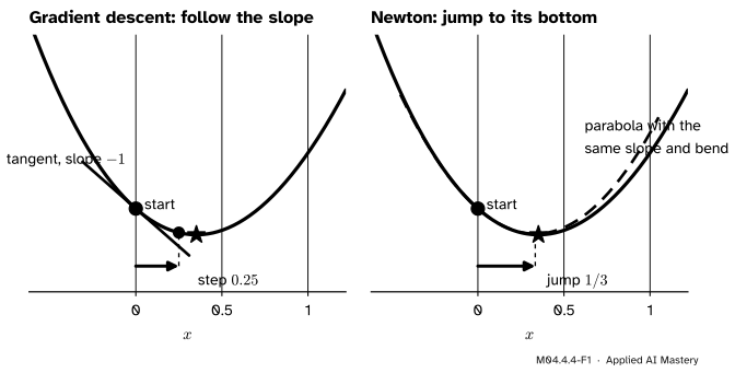
Stand on the curve at a point you can compute, \({x = 0}\). The tangent there has slope \({f'(0) = 0 - e^0 = -1}\): the ground falls to the right. So step right. Two questions remain: how far, and can the shape of the curve tell us more than a straight line can?
M04.4.4-F1
Two ways downhill from \({x = 0}\). Gradient descent steps against the slope, a distance proportional to it. Newton’s method fits the parabola with the same height, slope and bend, and jumps to its bottom, which lands almost on the star.
Gradient descent steps against the slope, and the steeper the ground, the longer the step. Newton’s method also uses the curvature: it fits the parabola that matches \(f\) in height, slope and bend at the current point, and jumps straight to the bottom of that parabola.
Build it up
Step 1. The local picture. For a small change \(s\), the linear approximation (M04.2.2) says
\[
f(x + s) \approx f(x) + f'(x)\,s .
\]
Step 2. Step against the slope. Choose \({s = -\eta f'(x)}\), with a small number \({\eta > 0}\) called the learning rate. Then
The change \({-\eta f'(x)^2}\) is negative whenever \({f'(x) \neq 0}\): a small step against the slope goes downhill, whichever way the slope points. Repeating it is gradient descent.
Step 3. Newton: aim for a flat point. We want a point where \({f' = 0}\). Apply the same linear approximation to the function \({f'}\), whose slope is \({f''}\):
\[
f'(x + s) \approx f'(x) + f''(x)\,s .
\]
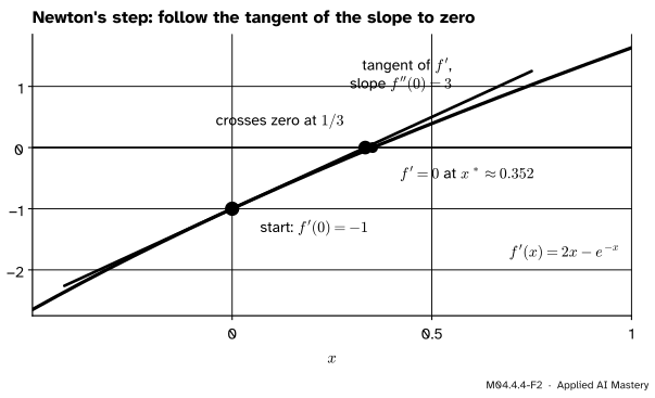
The right-hand side is zero when \({s = -f'(x)/f''(x)}\). That is Newton’s step: follow the tangent line of \({f'}\) to where it crosses zero.
M04.4.4-F2
Newton’s step seen on the graph of the slope. The tangent line of \({f'}\) at the start crosses zero at \({1/3}\), close to where \({f'}\) itself crosses zero, the bottom of \(f\).
Step 4. The same step, from the parabola. The parabola with the height, slope and bend of \(f\) at \(x\) is \({q(s)} = {f(x) + f'(x)s + \tfrac{1}{2}f''(x)s^2}\). Its slope \({f'(x) + f''(x)s}\) is zero at the same \(s\). When \({f''(x) > 0}\) that is the bottom of a cup; when \({f''(x) < 0}\), the top of a cap. This parabola is a Taylor polynomial, met properly in M04.8.3.
The formal statement
NoteDefinitions: gradient descent and Newton’s method
Start at \({x_0}\). Gradient descent with learning rate \({\eta > 0}\) repeats
Both stand still exactly where \({f' = 0}\): at a critical point. With small enough steps, gradient descent at least moves downhill on the way there; Newton’s step heads for the top of a cap wherever \({f'' < 0}\).
Small steps go downhill. If \({f'(x) \neq 0}\), then \({f(x - \eta f'(x)) < f(x)}\) for every small enough \({\eta > 0}\) (proved in the block below). How small is small enough depends on the curvature. On the running loss, with \({L'(w) = 15w - 23.5}\), a learning rate of 0.05 takes \({w = 0}\) to 1.175, 1.469 and 1.542, closing in on \({47/30 \approx 1.567}\) from one side. With 0.12 the first step lands at 2.82, past the bottom. Lesson ML01.5.3 works out exactly which learning rates converge.
Newton on a parabola takes one step. The running loss has \({L''(w) = 15}\), so from any \(w\)
\[
\begin{aligned}
&w - \frac{15w - 23.5}{15} \\
&\quad = w - w + \frac{23.5}{15} = \frac{47}{30} .
\end{aligned}
\]
Every start lands on the minimum at once, because the parabola Newton fits to \(L\) is \(L\) itself.
Go deeper: proof that a small enough step goes downhill
By the definition of the derivative, the ratio \({r = E(s)/s}\) tends to 0 as \({s \to 0}\). Put \({s = -\eta f'(x)}\). Then \({f'(x)s = -\eta f'(x)^2}\) and \({E(s)} = {rs} = {-\eta f'(x)\,r}\), so the change \({\Delta} = {f(x + s) - f(x)}\) is
As \({\eta \to 0}\), \(s\) and \(r\) shrink to 0, so \({f'(x)}\) times the bracket tends to \({f'(x)^2 > 0}\). Once it is positive, \(\Delta\) is \({-\eta}\) times a positive number: negative.
Worked example
Take steps of both methods on \({f(x) = x^2 + e^{-x}}\) from \({x_0 = 0}\), with \({\eta = 0.25}\) for gradient descent. We need \({f'(x) = 2x - e^{-x}}\) and \({f''(x) = 2 + e^{-x}}\).
Gradient descent.\({f'(0) = -1}\), so \({x_1} = {0 - 0.25 \times (-1)} = {0.25}\). Then \({f'(0.25)} = {0.5 - e^{-0.25}} = {0.5 - 0.7788} = {-0.2788}\), so
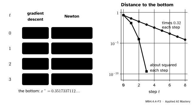
The first steps of both methods. Gradient descent shrinks the distance to the bottom by a steady factor; Newton’s method roughly squares it.
The bottom is at \({x^* \approx 0.351734}\), where \({f(x^*) \approx 0.8272}\). The distance of gradient descent from it runs 0.35, 0.10, 0.032, 0.010, cut each time by a factor that settles near 0.32. Newton’s runs 0.35, 0.018, 0.000044 and then about \({2.6 \times 10^{-10}}\): roughly squared at each step, so the number of correct digits roughly doubles. The speed has a price. Each Newton step needs the second derivative, which for a model with a million parameters becomes a table of a million times a million numbers (M08.5). That is why deep learning mostly uses gradient descent.
Code
From scratch, each method is a loop of one line:
import mathdef f(x):return x**2+ math.exp(-x)def f_slope(x):return2* x - math.exp(-x)def f_bend(x):return2+ math.exp(-x)def gradient_descent(slope, x, eta, steps): path = [x]for _ inrange(steps): x = x - eta * slope(x) path.append(x)return pathdef newton(slope, bend, x, steps): path = [x]for _ inrange(steps): x = x - slope(x) / bend(x) path.append(x)return pathgd = gradient_descent(f_slope, 0.0, 0.25, 30)nt = newton(f_slope, f_bend, 0.0, 4)print("gradient descent:", [round(x, 4) for x in gd[:4]], " after 30 steps:", round(gd[-1], 10))print("Newton: ", [round(x, 10) for x in nt])
The library call, scipy.optimize.minimize_scalar, uses Brent’s method by default and needs only \(f\) itself:
from scipy.optimize import minimize_scalarresult = minimize_scalar(f)print(f"minimize_scalar: x = {result.x:.7f}, f(x) = {result.fun:.7f}")
minimize_scalar: x = 0.3517337, f(x) = 0.8271840
On the running loss Newton needs one step from anywhere. On the double well the start decides the valley, and Newton from 0.3 runs to the peak:
loss_slope =lambda w: 15* w -23.5print("Newton on the running loss, one step from w = 0, 3, -1.7:", [newton(loss_slope, lambda w: 15.0, w0, 1)[1] for w0 in (0, 3, -1.7)])well =lambda x: x**4-2* x**2well_slope =lambda x: 4* x**3-4* xwell_bend =lambda x: 12* x**2-4for x0 in (-0.3, 0.3, 1.5):print(f"gradient descent (eta = 0.1) from {x0:4}: ends at {gradient_descent(well_slope, x0, 0.1, 200)[-1]:.4f}")print("Newton from 0.3:", [f"{x:.2e}"for x in newton(well_slope, well_bend, 0.3, 3)])print("minimize_scalar on the double well:", round(minimize_scalar(well).x, 4))print("minimize_scalar on the running cubic:", round(minimize_scalar(lambda x: x**3-3* x).x, 4))
Newton on the running loss, one step from w = 0, 3, -1.7: [1.5666666666666667, 1.5666666666666667, 1.5666666666666667]
gradient descent (eta = 0.1) from -0.3: ends at -1.0000
gradient descent (eta = 0.1) from  0.3: ends at 1.0000
gradient descent (eta = 0.1) from  1.5: ends at 1.0000
Newton from 0.3: ['3.00e-01', '-7.40e-02', '8.23e-04', '-1.12e-09']
minimize_scalar on the double well: 1.0
minimize_scalar on the running cubic: 1.0
Explore
M04.4-X1
Descent explorer
Choose a curve, then drag the ball or move it with the slider, and take gradient or Newton steps. Try the double well from 0.3 with both methods, and the running loss with a learning rate above 0.07, where every step overshoots.
Pitfalls
M04.4.4-F4
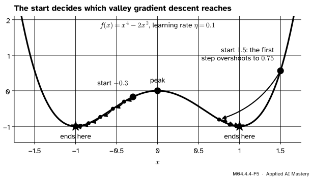
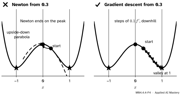
Wrong beside right, from the same start. Where \({f'' < 0}\), Newton’s parabola opens downward and its step heads for the peak; gradient descent walks down into a valley.
“Newton’s method finds the minimum.”
It finds a point where \({f' = 0}\), of any kind. On the double well from 0.3, where \({f''(0.3) = -2.92}\), its steps go to \({-0.074}\), then 0.0008, then the peak at 0. Check that \({f'' > 0}\) where it stops, or use a method that only moves downhill.
“Gradient descent finds the lowest point.”
It finds the valley that the start leads to. On the double well, with learning rate 0.1, starts between \({-1.5}\) and 0 end at \({-1}\) and starts between 0 and 1.5 end at 1. The library is no different: on the running cubic minimize_scalar reports \({x = 1}\) with value \({-2}\), a local minimum of a function that has no lowest point at all.
“A bigger learning rate is always faster.”
A step that is too big jumps past the bottom: on the running loss, 0.12 takes \({w = 0}\) to 2.82. Beyond a limit, worked out in ML01.5.3, the jumps grow and the run blows up.
Check yourself
Recall
1. Write the gradient-descent update and name \(\eta\).
Show answer
\({x_{t+1} = x_t - \eta f'(x_t)}\). \(\eta\) is the learning rate.
2. Why does a small step against the slope go downhill?
Show answer
By the linear approximation the change is about \({-\eta f'(x)^2}\), which is negative whenever \({f'(x) \neq 0}\).
3. Write Newton’s update, and say where it comes from.
Show answer
\({x_{t+1}} = {x_t - f'(x_t)/f''(x_t)}\): the point where the tangent line of \({f'}\) crosses zero, or equally the bottom of the parabola with the same height, slope and bend.
4. Why does Newton’s method reach the minimum of the running loss in one step?
Show answer
\({L'}\) is a straight line, so its tangent line is \({L'}\) itself, and following it to zero lands exactly on \({47/30}\).
5. Why can Newton’s method from 0.3 end at the peak of the double well?
Show answer
There \({f''(0.3) < 0}\), so its parabola opens downward and the step goes to the top. Newton’s method looks for \({f' = 0}\), not for a minimum.
Exercises
1.★ From \({w = 1}\) on the running loss, take one gradient-descent step with \({\eta = 0.05}\) and one Newton step. Compare both with \({47/30 \approx 1.5667}\).
2.★★ For \({f(x) = x - \ln x}\) with \({x > 0}\), show that Newton’s step is \({x \mapsto 2x - x^2}\) and that the distance to the minimum at 1 is squared at every step. What happens from \({x_0 = 2}\)?
Show solution
\({f'(x) = 1 - 1/x}\) and \({f''(x) = 1/x^2}\), so the step is \({(1 - 1/x)\,x^2 = x^2 - x}\) and the new point is \({x - (x^2 - x) = 2x - x^2}\). Then \({1 - (2x - x^2)} = {1 - 2x + x^2} = {(1 - x)^2}\): the new distance is the old one squared. From 0.5 the distances are 0.5, 0.25, 0.0625, 0.0039. From 2 the distance 1 squares to 1 again, and indeed \({2 \times 2 - 4 = 0}\): the step lands on \({x = 0}\), where \({\ln x}\) is not defined. Newton’s method can jump out of the domain.
3.★★★ Show that one Newton step on any parabola \({f(x) = ax^2 + bx + c}\) with \({a > 0}\) lands on its lowest point \({-b/(2a)}\) from every start, and that gradient descent with \({\eta = 1/(2a)}\) does the same. Why can no single learning rate do this for every parabola?
Show solution
\({f'(x) = 2ax + b}\) and \({f''(x) = 2a}\), so Newton gives \({x - (2ax + b)/(2a)} = {-b/(2a)}\), the lowest point found by completing the square (M01.3.3). Gradient descent gives \({x - \eta(2ax + b)}\), which is the same expression when \({\eta = 1/(2a)}\). So Newton’s method is gradient descent with the learning rate \({1/f''}\), chosen afresh from the curvature at every step. A fixed \(\eta\) matches only one curvature: on a parabola with a different \(a\) it falls short or jumps past the bottom.
Summary card
When \({f' = 0}\) has no formula, search: step against the slope, or jump to the bottom of the fitted parabola.
M04.4.4-F1
Two ways downhill.
Gradient descent: \({x_{t+1} = x_t - \eta f'(x_t)}\); a small step lowers \(f\) by about \({\eta f'(x_t)^2}\).
Newton: \({x_{t+1}} = {x_t - f'(x_t)/f''(x_t)}\), the zero of the tangent line of \({f'}\); one step on a parabola.
Newton’s error roughly squares at each step; gradient descent’s shrinks by a steady factor.
Both stop at any flat point. The start decides which, and Newton can head for a peak.
Sources and next steps
Sources. Each was opened and checked against this lesson on 12 November 2026.
Marc Peter Deisenroth, A. Aldo Faisal and Cheng Soon Ong, Mathematics for Machine Learning, Chapter 7. The introduction works a one-dimensional polynomial with two minima and a maximum (equations 7.1 to 7.3) and shows that the starting point decides which minimum the negative gradient leads to; Section 7.1 gives the gradient-descent update (7.6), which lowers the function for a small enough step size (7.5).
Stephen Boyd and Lieven Vandenberghe, Convex Optimization, Section 9.5.1: the Newton step minimises the second-order approximation (9.28), lands on the exact minimiser when the function is quadratic, and in one dimension is the zero of the linear approximation of \({f'}\) (Figure 9.18).
Gilbert Strang and Edwin Herman, Calculus Volume 1 (OpenStax), Section 4.9: Newton’s method for solving an equation (Equation 4.8), built from the tangent line, and the ways it fails. This lesson applies it to the equation \({f'(x) = 0}\).
David Jerison, MIT OpenCourseWare 18.01SC, Session 33, “Newton’s Method”: linear approximation used to make better and better guesses, and the cases where it does not work.
SciPy developers, scipy.optimize.minimize_scalar (SciPy 1.18 reference): Brent’s method by default, the Bounded method when bounds are given.
Next. This completes the module. M04.10, partial derivatives, may be read straight after it, and ML01.5.2 The gradient and the update rule takes gradient descent to a line with two parameters. The course continues with M04.5, integrals as accumulated area.