The slope of a function of a function is the product of the slopes of its links, as gear ratios multiply. Derived from the linear approximation, the chain rule gives the derivative of ln x, the power rule for every exponent, the slope of a squared error and the backward pass at the heart of backpropagation.
Explain the chain rule as gear ratios multiplying, and state it in prime notation and in Leibniz notation.
Derive the chain rule from the linear approximation of each link.
Use the chain rule to show that ln x has derivative 1/x and that the power rule holds for every real exponent.
Find the slope of the squared error of one example in its weight, and of a three-link chain through a sigmoid by multiplying local slopes from the output back.
In review. The maths and code on this page are checked by automated tests on every change, but an independent reader has not signed it off yet. Spot a mistake or a confusing step? Tell us.
The question
Every model in machine learning is a chain. A weight feeds a score, the score feeds an activation, the activation feeds a loss. Gradient descent needs one number: how fast the loss changes when the weight is nudged. The slope of each link on its own is easy. How do the slopes of the links combine into the slope of the whole chain?
From the last lesson
1. State the product rule.
Show answer
\({(f\,g)' = f'\,g + f\,g'}\): each function’s slope times the other function, added.
2. Write the slope of the sigmoid in terms of \(\sigma\). Where is it largest, and how large?
Show answer
\({\sigma'(z) = \sigma(z)\,(1 - \sigma(z))}\), largest at \({z = 0}\), where it is \(\tfrac14\).
Intuition
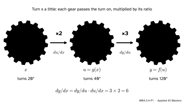
A function of a function, \({y = f(g(x))}\), is a chain of two links: \(x\) goes into the inner function \(g\) and comes out as \({u = g(x)}\), and \(u\) goes into the outer function \(f\) and comes out as \({y = f(u)}\) (composition, lesson M01.3.4). Picture each of the three quantities as a gear.
M04.3.4-F1
Turn \(x\) a little and \(u\) turns 2 times as far, so \(y\) turns 3 times as far as \(u\): 6 times as far as \(x\). Gear ratios multiply.
Turn the input gear a little. The \(u\) gear turns \({du/dx}\) times as far, and the \(y\) gear turns \({dy/du}\) times as far as \(u\). So \(y\) turns \({(dy/du) \cdot (du/dx)}\) times as far as \(x\). In the picture the ratios are 2 and 3 everywhere, because both links are straight lines, for example \({u = 2x + 1}\) and \({y = 3u - 2}\), which make \({y = 6x + 1}\).
For curved links the ratio changes from place to place. But close up, every smooth curve looks like its tangent line (M04.2.2), so near any point each gear has a definite local ratio: its slope there. The slope of the chain is the product of the local ratios, each read at the right place, the inner one at \(x\) and the outer one at \({u = g(x)}\). This is the chain rule.
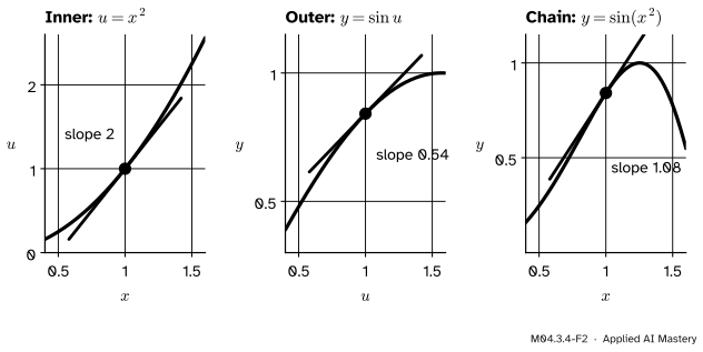
Step 2. Zoom in on curved links. Take \({y = \sin(x^2)}\) at \({x = 1}\). The inner link \({u = x^2}\) has slope 2 there, and it sends \({x = 1}\) to \({u = 1}\). The outer link \({y = \sin u}\) has slope \({\cos 1 \approx 0.54}\) at \({u = 1}\).
M04.3.4-F2
Each link, close up, is nearly its tangent line. The chain’s tangent at \({x = 1}\) has slope \({2 \times 0.54 = 1.08}\), the product.
Step 3. Chain the two tangent lines. A nudge \(h\) in \(x\) moves \(u\) by about \(2h\). A change of \(2h\) in \(u\) moves \(y\) by about \({0.54 \times 2h \approx 1.08\,h}\). So the slope of \({\sin(x^2)}\) at \({x = 1}\) is \({2\cos 1 \approx 1.08}\). Measured with a nudge of \({h = 0.001}\), the change in \(y\) is 0.001079, a ratio of about 1.079.
Step 4. Read each slope at its own point. The inner slope is read where the inner function works, at \(x\). The outer slope is read where the outer function works, at \({u = g(x)}\), not at \(x\).
The formal statement
NoteThe chain rule
If \(g\) has a derivative at \(x\) and \(f\) has a derivative at \({g(x)}\), then \({f(g(x))}\) has a derivative at \(x\), and
Derivation from the linear approximation. Let \({b = g(x)}\). Make the linear approximation of each link exact by naming its error. For the inner link, for \({h \neq 0}\), let \(\delta(h)\) be the gap between the secant slope and the tangent slope:
By the definition of \(g'(x)\), \(\delta(h)\) tends to 0 as \(h\) does. For the outer link, for every \({k \neq 0}\) let \(\varepsilon(k)\) be its gap in the same way, and set \({\varepsilon(0) = 0}\):
This now holds for every \(k\), including \({k = 0}\), where both sides are 0, and \(\varepsilon(k)\) tends to 0 as \(k\) does. Nudge \(x\) by \(h\) and let \({k = g(x + h) - g(x)}\), the change in \(u\). Then
Divide by \(h\). As \(h\) tends to 0, \(\delta(h)\) tends to 0; so does \({k = (g'(x) + \delta(h))\,h}\), and with it \(\varepsilon(k)\), since \(\varepsilon\) tends to \({\varepsilon(0) = 0}\) even when \(k\) is exactly 0. By the product law the quotient tends to \({f'(b)\,g'(x) = f'(g(x))\,g'(x)}\). Each factor is one gear ratio, plus an error that vanishes.
Go deeper: why not simply multiply and divide by the change in u?
A shorter argument writes the quotient as \({\tfrac{\Delta y}{\Delta u} \cdot \tfrac{\Delta u}{h}}\) and lets each factor tend to its slope. It is the right idea, and OpenStax gives it as an informal proof, but it breaks down when \({\Delta u = 0}\), which can happen for small nonzero \(h\) when the inner function is flat or wiggles. The error \(\varepsilon\), with \({\varepsilon(0) = 0}\), is the repair: it never divides by \(\Delta u\).
Consequence 1: the slope of \(\ln x\). For \({x > 0}\), \(\ln\) undoes \(e^x\) (lesson M01.4.3), so \({e^{\ln x} = x}\). Differentiate both sides. On the left the outer link is \(e^u\), whose slope is itself, and the inner link is \({u = \ln x}\):
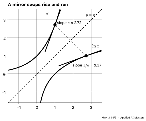
This assumes that \(\ln x\) has a slope, which the mirror picture below makes plain: the graph of \(\ln x\) is the graph of \(e^x\) reflected in the line \({y = x}\), the reflection swaps rise and run, and so each slope turns into its reciprocal.
M04.3.4-F3
The tangent to \(e^x\) at \({(1, e)}\) has slope \(e\); its mirror image touches \(\ln x\) at \({(e, 1)}\) with slope \({1/e}\).
Go deeper: a proof that ln x has a slope
Fix \({x > 0}\) and a small \({h \neq 0}\), and write \({y = \ln x}\) and \({k = \ln(x + h) - \ln x}\). Then \({x = e^y}\) and \({x + h = e^{y + k}}\), so \({h = e^{y+k} - e^y}\); and \({k \neq 0}\), because different inputs have different logarithms. The difference quotient of \(\ln\) is
As \(h\) shrinks so does \(k\), because the graph of \(\ln\) has no breaks: it is the mirror image of an unbroken graph. The bottom is then the difference quotient of \(e^x\) at \(y\), which tends to \({e^y = x}\). So \({k/h}\) tends to \({1/x}\): \(\ln x\) has a slope, and it is \({1/x}\).
Consequence 2: the power rule for every exponent. For \({x > 0}\) and any real \(r\), write \({x^r = (e^{\ln x})^r = e^{r \ln x}}\). The outer link is \(e^u\) and the inner link is \({u = r\ln x}\), with slope \({r/x}\):
So \({(\sqrt{x})' = \tfrac12 x^{-1/2} = 1/(2\sqrt{x})}\), which is \(\tfrac14\) at \({x = 4}\), the slope lesson M04.2.2 found by rationalising; and \({(x^{-1})' = -x^{-2}}\), as M04.2.3 found.
Consequence 3: the slope at 0 of \(a^x\). Since \({a^x = e^{x \ln a}}\), the chain rule gives \({(a^x)' = \ln a \cdot a^x}\). So the number \(m_a\) of lesson M04.3.2 is \(\ln a\): \({m_2 = \ln 2 \approx 0.693}\) and \({m_3 = \ln 3 \approx 1.099}\), as its table showed.
Go deeper: the e of lesson M04.3.2 is the e of lesson M01.4.2
Lesson M04.3.2 promised a proof that the base with slope 1 at 0 is the number that \({(1 + \tfrac1n)^n}\) settles towards. Take logarithms and put \({h = 1/n}\):
That is the difference quotient of \(\ln\) at 1, which tends to \({1/1 = 1}\) as \(n\) grows. So \({(1 + \tfrac1n)^n = e^{\,n \ln(1 + 1/n)}}\) tends to \({e^1 = e}\), because \(e^x\) has no breaks.
Worked example
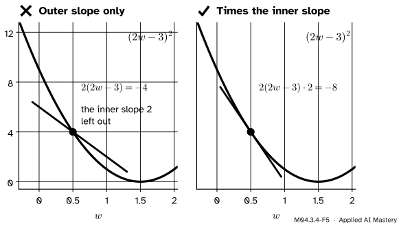
The squared error of one example. Take the second point of the running loss, \({(x, y) = (2, 3)}\), and the line \({\hat y = wx}\). Its squared error is \({E(w) = (wx - y)^2}\), a chain of two links: the residual \({r = wx - y}\), with slope \({dr/dw = x}\), then its square \({E = r^2}\), with slope \({dE/dr = 2r}\). So
At \({w = 0.5}\) the residual is \({1 - 3 = -2}\), and the slope is \({2 \cdot (-2) \cdot 2 = -8}\). At \({w = 1}\) it is \({2 \cdot (-1) \cdot 2 = -4}\).
The running loss is the mean of four such errors, so its slope is the mean of four such terms (lesson ML01.5.2 sums exactly these). At \({w = 1}\) the four terms are \(-2\), \(-4\), \(-12\) and \(-16\), whose mean is \(-8.5\): the slope \({L'(1)}\) of lesson M04.3.1.
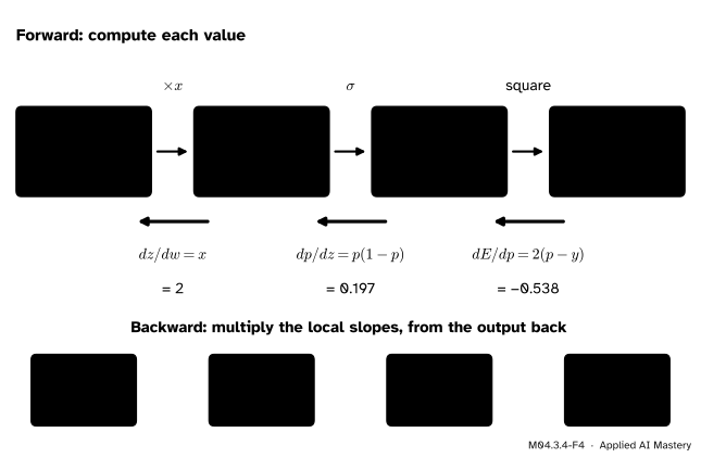
A three-link chain through a sigmoid. A classifier scores a positive example (target \({y = 1}\)) with input \({x = 2}\) as \({z = wx}\), turns the score into a probability \({p = \sigma(z)}\), and pays the squared error \({E = (p - y)^2}\). With \({w = 0.5}\), going forward: \({z = 1}\), \({p = \sigma(1) \approx 0.731}\) and \({E \approx 0.072}\).
Going backward, from the output, each link multiplies in its local slope. The slope of \(E\) in itself is 1. Times \({dE/dp = 2(p - y) \approx -0.538}\) gives the slope of \(E\) in \(p\). Times \({dp/dz = p(1 - p) \approx 0.197}\) (lesson M04.3.3) gives \(-0.106\), the slope in \(z\). Times \({dz/dw = x = 2}\) gives the slope in \(w\):
The worked chain. Values flow forward; slopes flow backward. Each yellow tag is the slope of the error in the value above it, the running product of the local slopes to its right.
The slope is negative, so raising \(w\) lowers the error: the score is pushed up, towards the target. Multiplying from the output back is the order a computer uses in backpropagation (M05.9): each running product is reused by every link before it, so one backward pass gives the slope in every weight of a network at once.
Code
From scratch: the slope of \({\sin(x^2)}\) at \({x = 1}\) as a product of two gear ratios, against the change measured for shrinking nudges.
import mathinner_ratio =2*1.0# du/dx = 2x at x = 1outer_ratio = math.cos(1.0**2) # dy/du = cos u at u = 1print("product of the ratios:", round(inner_ratio * outer_ratio, 6))for h in (0.1, 0.01, 0.001): measured = (math.sin((1+ h) **2) - math.sin(1)) / hprint(f"nudge h = {h:<6} measured change per unit of x: {measured:.6f}")
product of the ratios: 1.080605
nudge h = 0.1    measured change per unit of x: 0.941450
nudge h = 0.01   measured change per unit of x: 1.068937
nudge h = 0.001  measured change per unit of x: 1.079460
The squared error of each example and its slope \({2(wx - y)\,x}\), checked by a central difference, and averaged over the four points of the running loss:
import numpy as npX = np.array([1.0, 2.0, 3.0, 4.0])Y = np.array([2.0, 3.0, 5.0, 6.0])def error_slope(w, x, y):return2* (w * x - y) * xh =1e-6for w in (0.5, 1.0): central = (((w + h) *2-3) **2- ((w - h) *2-3) **2) / (2* h)print(f"w = {w}: rule {error_slope(w, 2.0, 3.0)}, central difference {central:.6f}")print("the four terms at w = 1:", error_slope(1.0, X, Y), " mean:", error_slope(1.0, X, Y).mean())w = np.linspace(0, 3, 7)means = np.array([error_slope(v, X, Y).mean() for v in w])print("mean term equals 15w - 23.5 at seven weights:", np.allclose(means, 15* w -23.5))
w = 0.5: rule -8.0, central difference -8.000000
w = 1.0: rule -4.0, central difference -4.000000
the four terms at w = 1: [ -2.  -4. -12. -16.]  mean: -8.5
mean term equals 15w - 23.5 at seven weights: True
The three-link chain, forward then backward, exactly as in the figure. Each step of the backward pass multiplies the running product by one local slope:
def sigmoid(z):return1/ (1+ math.exp(-z))w, x, y =0.5, 2.0, 1.0z = w * x # forwardp = sigmoid(z)E = (p - y) **2slope =1.0# backward: dE/dEslope *=2* (p - y) # dE/dpat_p = slopeslope *= p * (1- p) # dE/dzat_z = slopeslope *= x # dE/dwprint(f"forward: z = {z}, p = {p:.3f}, E = {E:.3f}")print(f"backward: dE/dp = {at_p:.3f}, dE/dz = {at_z:.3f}, dE/dw = {slope:.3f}")def error_of(w):return (sigmoid(w * x) - y) **2print("central difference in w:", round((error_of(w +1e-6) - error_of(w -1e-6)) /2e-6, 4))
forward:  z = 1.0, p = 0.731, E = 0.072
backward: dE/dp = -0.538, dE/dz = -0.106, dE/dw = -0.212
central difference in w: -0.2115
Last, the two consequences, checked by SciPy’s derivative: the slope of \(\ln x\) against \({1/x}\), and the power rule for exponents that are not whole numbers. SciPy samples the function on both sides of each point, starting half a unit away by default; near 0 that would reach inputs where \(\ln x\) and \(x^r\) are not defined, so the first step is set smaller here.
from scipy.differentiate import derivativexs = np.array([1.0, 2.0, 3.0, 4.0])print("ln:", np.round(derivative(np.log, xs, initial_step=0.2).df, 6), " 1/x:", np.round(1/ xs, 6))for r in (0.5, -1.0, 2.5, math.pi): slopes = derivative(lambda t: t ** r, xs, initial_step=0.2).dfprint(f"r = {r:.4f}: largest gap to r x^(r-1) is {np.max(np.abs(slopes - r * xs ** (r -1))):.1e}")print("slope of sqrt at 4:", round(float(derivative(np.sqrt, 4.0).df), 6))
ln: [1.       0.5      0.333333 0.25    ]   1/x: [1.       0.5      0.333333 0.25    ]
r = 0.5000: largest gap to r x^(r-1) is 3.7e-14
r = -1.0000: largest gap to r x^(r-1) is 2.5e-12
r = 2.5000: largest gap to r x^(r-1) is 2.8e-13
r = 3.1416: largest gap to r x^(r-1) is 7.1e-13
slope of sqrt at 4: 0.25
Explore
M04.3-X1
Chain-rule gears
Choose an inner and an outer function, then turn the input \(x\): drag the orange gear, use the slider, or step with the buttons. The two gear ratios are printed between the gears, and the read-out compares their product with the change in \(y\) measured for a small nudge \(h\).
Three things to find. With \({u = x^2}\), turn \(x\) upwards through 0: the middle gear turns backwards while \(x\) is negative, stops for a moment at 0, then turns forwards, and while its ratio is 0 the \(y\) gear stops too, whatever the outer function. With the outer function \({\sigma(u)}\), the last ratio never passes 0.25. And with any pair, shrink the nudge \(h\) and watch the measured \({\Delta y / \Delta x}\) close in on the product of the two ratios.
Pitfalls
M04.3.4-F5
Wrong beside right, for the squared error of the point \({(2, 3)}\). Without the inner slope the line is half as steep as the curve.
“The slope of \(f(g(x))\) is \(f'(g(x))\).”
That is the outer gear’s ratio alone. The inner gear’s ratio is missing. For the squared error \({(wx - y)^2}\) the outer slope \({2(wx - y)}\) without the factor \(x\) gives \(-4\) instead of \(-8\) at \({w = 0.5}\). In training, each example’s push would be off by a factor of its own input \(x\).
“Read the outer slope at \(x\).”
The outer function acts on \(u\), so its slope is read at \({u = g(x)}\). For \({\sin(x^2)}\) at \({x = 1.5}\) the right slope is \({\cos(2.25) \cdot 3 \approx -1.88}\); reading \(\cos\) at \(x\) gives \({\cos(1.5) \cdot 3 \approx 0.21}\), with the wrong sign. At \({x = 1}\) the two agree only by accident, because \({1^2 = 1}\).
“The Leibniz form is just cancelling \(du\), so it needs no proof.”
\({dy/du \cdot du/dx}\) looks like fractions cancelling, which makes it easy to remember. But \({du/dx}\) is one symbol, a limit, not a fraction, and the proof has to cope with \({\Delta u = 0}\). Use the form freely; know that it is a theorem.
Check yourself
Recall
1. State the chain rule in prime notation and in Leibniz notation.
Show answer
\({(f(g(x)))' = f'(g(x))\,g'(x)}\); with \({u = g(x)}\) and \({y = f(u)}\), \({dy/dx = dy/du \cdot du/dx}\).
2. In the gear picture, what happens to the \(y\) gear when the \(u\) gear’s ratio is 0?
Show answer
It stops too: \({dy/dx = dy/du \cdot 0 = 0}\), whatever the outer ratio is.
3. What is the derivative of \(\ln x\), and how does the chain rule find it?
Show answer
\({1/x}\). Differentiate both sides of \({e^{\ln x} = x}\): \({e^{\ln x} \cdot (\ln x)' = 1}\), so \({(\ln x)' = 1/e^{\ln x} = 1/x}\).
4. What is the slope in \(w\) of the squared error \({(wx - y)^2}\)?
Show answer
\({2(wx - y)\,x}\): twice the residual, times the input.
5. In the backward pass, in what order are the local slopes multiplied, and what does each running product mean?
Show answer
From the output back. Each running product is the slope of the output in the value it has reached, and the next link multiplies it by one more local slope.
Exercises
1.★ Differentiate \({(2x + 1)^4}\) and the bell curve \({e^{-x^2/2}}\), and find each slope at \({x = 1}\).
Show solution
For \({(2x + 1)^4}\) the outer link is \(u^4\) with slope \(4u^3\), and the inner link \({2x + 1}\) has slope 2: the derivative is \({4(2x + 1)^3 \cdot 2 = 8(2x + 1)^3}\), which is \({8 \cdot 27 = 216}\) at \({x = 1}\). For \({e^{-x^2/2}}\) the outer link is \(e^u\) and the inner link \({-x^2/2}\) has slope \({-x}\): the derivative is \({-x\,e^{-x^2/2}}\), which is \({-e^{-1/2} \approx -0.607}\) at \({x = 1}\).
2.★★ The softplus is \({\ln(1 + e^z)}\). Show that its derivative is the sigmoid \(\sigma(z)\), and find its slope at \({z = 0}\).
Show solution
The outer link is \(\ln u\) with slope \({1/u}\), and the inner link \({u = 1 + e^z}\) has slope \(e^z\). So the derivative is \({\tfrac{1}{1 + e^z} \cdot e^z = \tfrac{e^z}{1 + e^z} = \sigma(z)}\), the sigmoid written as in lesson M04.3.3. At \({z = 0}\) it is \({\sigma(0) = \tfrac12}\).
3.★★★ For a positive example the log loss is \({-\ln p}\), with \({p = \sigma(z)}\) and \({z = wx}\). Use the chain rule with three links to show that its slope in \(w\) is \({(p - 1)\,x}\). At \({w = 0.5}\) and \({x = 2}\), compare it with the squared-error chain of the worked example.
Show solution
The three local slopes are \({-1/p}\) for \({-\ln p}\), \({p(1 - p)}\) for the sigmoid, and \(x\) for \({z = wx}\). Their product is
At \({w = 0.5}\), \({x = 2}\): \({p \approx 0.731}\) and the slope is \({(0.731 - 1) \cdot 2 \approx -0.538}\), about 2.5 times the push of the squared error, \(-0.212\). The factor \({p(1 - p)}\) has cancelled, so this slope does not fade in the sigmoid’s flat tails: one reason logistic regression uses the log loss (lesson ML01.6.3).
Summary card
The slope of a chain is the product of the slopes of its links.
M04.3.4-F1
Gear ratios multiply.
\({(f(g(x)))' = f'(g(x))\,g'(x)}\), or \({dy/dx = dy/du \cdot du/dx}\).
\({(\ln x)' = 1/x}\) and \({(x^r)' = r\,x^{r-1}}\) for every real \(r\) and \({x > 0}\).
\({(wx - y)^2}\) has slope \({2(wx - y)\,x}\) in \(w\).
Backward pass: multiply the local slopes from the output back.
Sources and next steps
Sources. Each was opened and checked against this lesson on 12 November 2026.
Gilbert Strang and Edwin Herman, Calculus Volume 1, OpenStax: Section 3.6 states the chain rule (equation 3.17) with an informal proof that divides by \({g(x) - g(a)}\), and gives the rule for three functions and the Leibniz form; Section 3.9 finds the derivative of \(\ln x\) by differentiating \({e^y = x}\) (Theorem 3.15) and gives \({b^x \ln b}\) as the derivative of \(b^x\) (Theorem 3.16).
Matthew Boelkins, Active Calculus, Section 2.5, The chain rule. Names the inner and the outer function, and reads the rule as the derivative of the outer function, evaluated at the inner function, times the derivative of the inner function.
Marc Peter Deisenroth, A. Aldo Faisal and Cheng Soon Ong, Mathematics for Machine Learning: the chain rule (equation 5.32) and Example 5.5, which differentiates \({(2x + 1)^4}\) as in exercise 1; Section 5.6 presents backpropagation as reverse-mode automatic differentiation, through intermediate variables (Example 5.14).
Ian Goodfellow, Yoshua Bengio and Aaron Courville, Deep Learning, Chapter 6, Section 6.5.2: back-propagation is an algorithm that computes the chain rule with a highly efficient order of operations, and the rule \({dz/dx = dz/dy \cdot dy/dx}\) is equation 6.44.
Next. The rules of this module are the tools of module M04.4, which finds where a slope is zero, and of M04.10, which takes partial derivatives with them. In machine learning, lesson ML01.5.2 uses the chain rule to build gradient descent for a line.