Zoom in on a smooth curve and it straightens into its tangent line. Write that line from the derivative, estimate a square root with it by hand, watch its error shrink like the square of the step, and read the slope of a loss as the sensitivity behind every gradient step.
Write the equation of the tangent line to a graph at a point from the value and the derivative there.
Use the linear approximation f(a + h) ≈ f(a) + f’(a) h to estimate a value by hand, and say when it can be trusted.
Show that the error of the linear approximation shrinks like h squared, exactly for x squared and for the square root near 4.
Read the derivative of a loss as a sensitivity, and predict how a small change in a weight changes the loss.
In review. The maths and code on this page are checked by automated tests on every change, but an independent reader has not signed it off yet. Spot a mistake or a confusing step? Tell us.
The question
Without a calculator, what is \({\sqrt{4.1}}\) to three decimal places? You know that \({\sqrt{4} = 2}\), and 4.1 is close to 4. The trick that answers this in one line is the same one a model uses before it moves a weight: it predicts how much the loss will change.
From the last lesson
1. For \({f(x) = x^2}\), what is the secant slope from 1 to \({1 + h}\)?
Show answer
\({2 + h}\), for every \({h \neq 0}\). Its limit, 2, is \({f'(1)}\).
2. In words, what does \({f'(a)}\) measure?
Show answer
The limit of the secant slopes as the second point slides in: the slope of the tangent at \(a\), and the instantaneous rate of change of \(f\) at \(a\).
Intuition
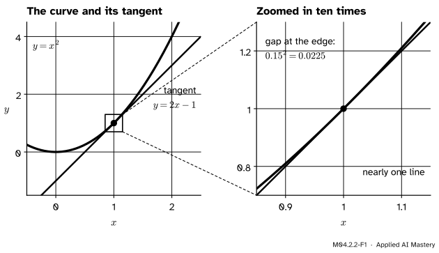
Zoom in on a smooth curve at one of its points and it looks straighter and straighter. Below, the running curve \({y = x^2}\) is seen near \({(1, 1)}\) through a window ten times smaller in each direction. Inside the window the curve is hard to tell from the straight line \({y = 2x - 1}\).
M04.2.2-F1
Zoom in on a smooth curve and it becomes a straight line: its tangent. At the edges of the right-hand window the curve has drifted only \({0.15^2 = 0.0225}\) from the tangent, under 4 per cent of the window’s height.
The line the curve turns into is its tangent line: it passes through the point and its slope is the derivative there, \({f'(1) = 2}\) for this curve. Zoom in ten times again and the drift at the edges falls from 0.0225 to 0.000225, a hundred times less in a window only ten times smaller. Near the point, the tangent is a stand-in for the curve, and a straight line is easy to compute with. That is the whole idea of this lesson.
Build it up
Step 1. A line from a point and a slope. In M01.3.2 the line with slope \(m\) through \({(x_0, y_0)}\) is \({y = mx + b}\) with intercept \({b = y_0 - mx_0}\). Put that \(b\) in and regroup: \({y = y_0 + m\,(x - x_0)}\). Start at the point and add slope times run. For the tangent at \(a\), the point is \({(a, f(a))}\) and the slope is \({f'(a)}\), so its equation is \({y = f(a) + f'(a)\,(x - a)}\).
Step 2. The tangent to the running curve. For \({f(x) = x^2}\) at \({a = 1}\), \({f(1) = 1}\) and \({f'(1) = 2}\), so the tangent is \({y = 1 + 2(x - 1)}\), which tidies to \({y = 2x - 1}\).
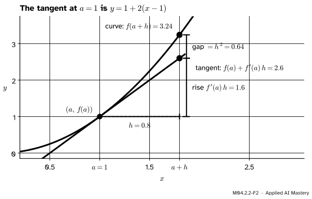
Step 3. Use the line instead of the curve. A step \(h\) from the point, at \({x = 1 + h}\), the tangent has height \({1 + 2h}\). With \({h = 0.1}\) that is 1.2, while the curve has height \({1.1^2 = 1.21}\). The line misses by 0.01.
M04.2.2-F2
The tangent at \({a = 1}\), followed a step \({h = 0.8}\): it rises \({f'(a)\,h = 1.6}\) to 2.6, while the curve reaches 3.24. The gap is \({h^2 = 0.64}\). A large step makes the gap easy to see.
Step 4. The gap is exactly \({h^2}\). Subtract the tangent’s height from the curve’s: \({(1 + h)^2 - (1 + 2h) = h^2}\). So the gap is 0.01 when \({h = 0.1}\) and 0.0025 when \({h = 0.05}\). Halve the step and the gap is quartered. Compare lesson 1, where the secant slope \({2 + h}\) missed the derivative by \(h\), which only halves.
The formal statement
NoteDefinition: tangent line and linear approximation
If \(f\) is differentiable at \(a\), its tangent line at \(a\) is
\[
y = f(a) + \cgrad{f'(a)}\,(x - a) .
\]
For \(x\) near \(a\), written \({x = a + h}\), the value of \(f\) is close to the tangent’s height:
The right-hand side is the linear approximation of \(f\) at \(a\).
Why the error is small. By the definition of the derivative, the difference quotient differs from \({f'(a)}\) by an amount that tends to 0. Call that amount \({r(h)}\):
So the error of the linear approximation is exactly \({h\,r(h)}\): the step times a number that itself shrinks to 0. Divide it by \(h\) and what is left, \({r(h)}\), tends to 0. In words, the error shrinks faster than the step. For \({x^2}\) at 1, lesson 1 found the quotient \({2 + h}\), so \({r(h) = h}\) and the error is \({h \cdot h = h^2}\), as in Step 4.
Go deeper: the tangent is the only line that does this
Take any other line through \({(a, f(a))}\), with a slope \({m \neq f'(a)}\). At \({a + h}\) it misses the curve by
Divided by \(h\) this tends to \({f'(a) - m}\), which is not 0. So every other line through the point misses by about a fixed multiple of \(h\), while the tangent misses by a vanishing multiple of \(h\). Near the point, the tangent is the best straight-line fit there is.
The slope of \({\sqrt{x}}\) at 4. For the worked example we need \({f'(4)}\) for \({f(x) = \sqrt{x}}\). The quotient \({(\sqrt{4+h} - 2)/h}\) is \({0/0}\) at \({h = 0}\), and this time there is no power to multiply out. Instead multiply top and bottom by \({\sqrt{4+h} + 2}\), which is not zero, and use \({(u - v)(u + v) = u^2 - v^2}\) (rationalising, M04.1.2):
The last line cancels \(h\). As \(h\) tends to 0, \({\sqrt{4+h}}\) tends to \({\sqrt{4} = 2}\) by the root law of M04.1.2, so the quotient tends to \({1/(2 + 2) = 1/4}\). The tangent to \({\sqrt{x}}\) at 4 is \({y = 2 + (x - 4)/4}\).
Worked example
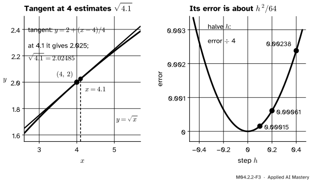
Estimate \({\sqrt{4.1}}\) by hand. Take \({a = 4}\) and \({h = 0.1}\) in the linear approximation:
A calculator gives \({\sqrt{4.1} = 2.02485}\) to five places, so the estimate is too big by about 0.00015, and it is right to three decimal places.
How big is the error, exactly? Let \({E(h) = 2 + h/4 - \sqrt{4 + h}}\), the amount by which the tangent overestimates. Squaring the tangent’s height gives \({(2 + h/4)^2 = 4 + h + h^2/16}\), which is \({h^2/16}\) more than \({(\sqrt{4+h})^2 = 4 + h}\). By \({u^2 - v^2 = (u - v)(u + v)}\), with \({u = 2 + h/4}\) and \({v = \sqrt{4+h}}\),
For small \(h\) the bottom is close to \({2 + 0 + 2 = 4}\), so \({E(h) \approx h^2/64}\). For \({h = 0.1}\) that is \({0.01/64 \approx 0.000156}\), against the true 0.000154. The bottom is positive for every \({h \ge -4}\), so \({E(h) > 0}\) whenever \({h \neq 0}\): away from 4 the tangent always overestimates the square root, and the curve bends away below its tangent.
\(h\)
error \({E(h)}\)
\({E(h)/h^2}\)
0.4
0.002382
0.01489
0.2
0.000610
0.01525
0.1
0.000154
0.01543
0.05
0.000039
0.01553
Each halving of \(h\) divides the error by almost exactly 4, and the last column creeps up on \({1/64 \approx 0.0156}\), as \({E(h) \approx h^2/64}\) says.
M04.2.2-F3
The worked example as a trace. The tangent at 4 gives 2.025 for \({\sqrt{4.1}}\) (left); its error, about \({h^2/64}\), is a quarter as large each time the step is halved (right).
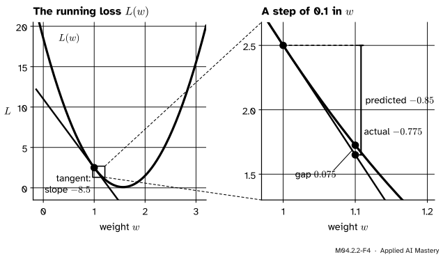
The derivative as a sensitivity. The same approximation answers a question about a model. The running loss of this course, the mean squared error of the line \({y = wx}\) on four points (ML01.5.1), is \({L(w) = 7.5w^2 - 23.5w + 18.5}\). Exercise 3 of lesson 1 gives its derivative, \({L'(w) = 15w - 23.5}\). At \({w = 1}\) the loss is \({L(1) = 2.5}\) and the slope is \({L'(1) = -8.5}\). The linear approximation reads
\[
\Delta L \approx L'(w)\,\Delta w ,
\]
where \({\Delta w}\) is a small change in the weight and \({\Delta L}\) the change it causes in the loss. Move \(w\) from 1 to 1.1: the prediction is \({-8.5 \times 0.1 = -0.85}\). The true change is \({L(1.1) - L(1)} = {1.725 - 2.5} = {-0.775}\). With \({\Delta w = 0.01}\) the prediction is \({-0.085}\) and the truth \({-0.08425}\). The gap is \({7.5\,\Delta w^2}\) each time, so it shrinks with the square of the step, as it must.
M04.2.2-F4
The slope of the loss as a sensitivity. From \({w = 1}\), a step of 0.1 changes the loss by about the slope times the step, \({-0.85}\); the true change is \({-0.775}\).
This is how training reads a derivative. The slope says how sensitive the loss is to the weight, and its sign says which way the loss goes. Here the slope is negative, so increasing \(w\) lowers the loss. Choose the step \({\Delta w = -\eta\, L'(w)}\) for a small positive number \(\eta\), the learning rate. Then \({\Delta L \approx -\eta\, L'(w)^2}\), which is never positive. That is one step of gradient descent, which ML01.5.2 builds on.
Code
First from scratch: build the tangent line as a function, and measure its error against the square root.
import mathdef tangent_line(f, a, slope):"""The tangent to f at a, as a function of x: f(a) + slope * (x - a)."""returnlambda x: f(a) + slope * (x - a)T = tangent_line(math.sqrt, 4, 0.25)print(f"tangent at 4.1: {T(4.1):.6f}")print(f"sqrt(4.1): {math.sqrt(4.1):.6f}")print(" h error error / h^2")for h in [0.4, 0.2, 0.1, 0.05, 0.025]: error = T(4+ h) - math.sqrt(4+ h)print(f" {h:<7}{error:.6f}{error / h**2:.5f}")
The ratio settles on 0.0156, which is \({1/64}\). The slope 0.25 was found by algebra; the quotient of lesson 1 confirms it, creeping up on 0.25 as the step shrinks.
for h in [0.1, 0.01, 0.001]:print(f"h = {h:<6}{(math.sqrt(4+ h) -2) / h:.6f}")
h = 0.1    0.248457
h = 0.01   0.249844
h = 0.001  0.249984
Now the sensitivity of the loss, with NumPy doing several steps at once.
import numpy as npdef L(w):return7.5* w**2-23.5* w +18.5# the running lossdef dL(w):return15* w -23.5# its derivativesteps = np.array([0.1, 0.01, 0.001])predicted = dL(1.0) * stepsactual = L(1.0+ steps) - L(1.0)print("dw predicted actual gap")for dw, p, a inzip(steps, predicted, actual):print(f"{dw:<6}{p:+.4f}{a:+.5f}{a - p:.7f}")
dw     predicted actual    gap
0.1    -0.8500   -0.77500  0.0750000
0.01   -0.0850   -0.08425  0.0007500
0.001  -0.0085   -0.00849  0.0000075
The gap column is \({7.5\,\Delta w^2}\): 0.075, 0.00075 and 0.0000075.
Explore
This module’s interactive, the secant slider, lives in lesson M04.2.1. Choose \({x^2}\) at 1 and press Zoom in three times: the curve flattens onto the green tangent, and the read-out reports how wide the window has become. Then choose \({\sqrt{x}}\) at 4, where the tangent is the one this lesson used to estimate \({\sqrt{4.1}}\). Last, choose \({\abs{x}}\) at 0 and zoom: the corner never straightens, and the next lesson explains why.
Pitfalls
M04.2.2-F5
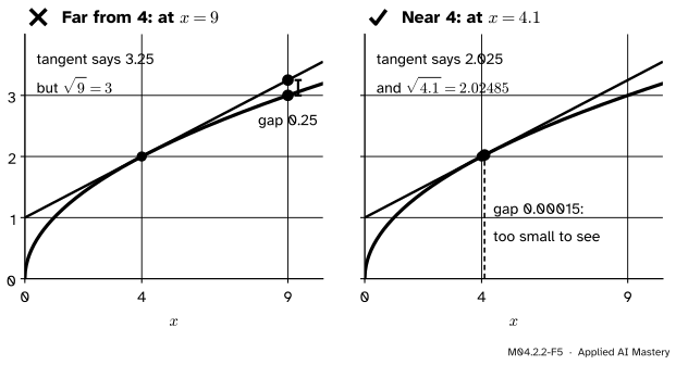
Wrong beside right. Used five units from 4, the tangent misses \({\sqrt{9}}\) by 0.25. Used a tenth of a unit away, it misses \({\sqrt{4.1}}\) by 0.00015.
“The tangent line approximation is good everywhere.”
It is good near \(a\) only. Close to \(a\) its error grows like the square of the distance, and far away it can be large. The tangent to \({\sqrt{x}}\) at 4 gives \({2 + 5/4 = 3.25}\) at \({x = 9}\), where the truth is 3. To estimate \({\sqrt{9.2}}\), use the tangent at 9 instead (exercise 2).
“The tangent line at \(a\) is \({y = f'(a)\,x + f(a)}\).”
That line has the right slope but passes through \({(0, f(a))}\), not through \({(a, f(a))}\). For \({x^2}\) at 1 it would be \({y = 2x + 1}\), which misses the point \({(1, 1)}\) by 2. The shift \({x - a}\) is what makes the line pass through the point: \({y = f(a) + f'(a)\,(x - a)}\).
“A tangent touches a curve at one point and never crosses it.”
That is true of circles, not of graphs in general. The tangent to \({y = x^3}\) at 0 is the line \({y = 0}\) (the quotient \({h^3/h = h^2}\) tends to 0), and the curve crosses it there. The running cubic of this course, \({g(x) = x^3 - 3x}\), has the quotient \({3h + h^2}\) at \({x = 1}\), so its tangent there is the flat line \({y = g(1) = -2}\). That line meets the curve again at \({x = -2}\), since \({(-2)^3 - 3(-2) = -2}\). A tangent is defined by its slope at the point, not by touching once.
“To lower the loss, move the weight in the direction of the slope.”
The other way. At \({w = 1}\) the slope \({L'(1) = -8.5}\) is negative, so the loss falls as \(w\) grows: lower it by increasing \(w\), against the sign of the slope. Stepping with the slope climbs the loss, which is why the gradient step subtracts \({\eta\, L'(w)}\).
Check yourself
Recall
1. Write the equation of the tangent line to the graph of \(f\) at \({x = a}\).
Show answer
\({y = f(a) + f'(a)\,(x - a)}\).
2. State the linear approximation of \({f(a + h)}\).
Show answer
\({f(a + h) \approx f(a) + f'(a)\,h}\), good for small \(h\).
3. What is the tangent to \({y = x^2}\) at \({x = 1}\)?
Show answer
\({y = 1 + 2(x - 1)}\), that is \({y = 2x - 1}\).
4. For \({x^2}\) at 1, what happens to the error of the linear approximation when \(h\) is halved?
Show answer
It is quartered: the error is exactly \({h^2}\).
5. The running loss has \({L'(1) = -8.5}\). About how much does the loss change when \(w\) moves from 1 to 1.02?
Show answer
By about \({-8.5 \times 0.02 = -0.17}\): it falls by about 0.17.
Exercises
1.★ Write the tangent to \({y = x^2}\) at \({x = 3}\), and use it to estimate \({3.1^2}\). What is the error?
Show solution
From lesson 1 (exercise 3 with \({p = 1}\), \({q = 0}\)), \({f'(3) = 6}\), and \({f(3) = 9}\). The tangent is \({y = 9 + 6(x - 3) = 6x - 9}\). At 3.1 it gives \({9 + 6 \times 0.1 = 9.6}\), while \({3.1^2 = 9.61}\). The error is \({0.01 = h^2}\), as for every point of \({x^2}\): \({(a + h)^2 - (a^2 + 2ah) = h^2}\).
2.★★ Estimate \({\sqrt{3.9}}\) with the tangent at 4. Then find the slope of \({\sqrt{x}}\) at 9 from the definition, and use it to estimate \({\sqrt{9.2}}\).
Deduce that \({E(h) \approx h^2/(8a\sqrt{a})}\) for small \(h\), and check that this is \({h^2/64}\) at \({a = 4}\).
Show solution
The quotient rationalises as before: \({(\sqrt{a+h} - \sqrt{a})/h} = {1/(\sqrt{a+h} + \sqrt{a})}\), which tends to \({1/(2\sqrt{a})}\). So the tangent’s height at \({a + h}\) is \({u = \sqrt{a} + h/(2\sqrt{a})}\), and
\[
\begin{aligned}
u^2 &= a + h + \frac{h^2}{4a} , \\
u^2 - (\sqrt{a+h})^2 &= \frac{h^2}{4a} .
\end{aligned}
\]
Factor the left side as \({(u - \sqrt{a+h})(u + \sqrt{a+h})}\) and divide by the second factor, which is positive, to get the formula for \({E(h) = u - \sqrt{a+h}}\). As \(h\) tends to 0 the bottom tends to \({2\sqrt{a}}\), so \({E(h)} \approx {h^2/(4a \cdot 2\sqrt{a})} = {h^2/(8a\sqrt{a})}\). At \({a = 4}\) this is \({h^2/(8 \times 4 \times 2) = h^2/64}\).
Summary card
Near a point, a smooth curve is its tangent line.
M04.2.2-F1
Zoom in and the curve straightens.
Tangent line.\({y = f(a) + f'(a)\,(x - a)}\).
Linear approximation.\({f(a + h) \approx f(a) + f'(a)\,h}\), with an error that shrinks faster than \(h\).
By hand.\({\sqrt{4.1} \approx 2.025}\) (truth 2.02485); the error is about \({h^2/64}\).
Sensitivity.\({\Delta L \approx L'(w)\,\Delta w}\); for the running loss \({L'(1) = -8.5}\), so stepping up \(w\) lowers \(L\).
Sources and next steps
Sources. Each was opened and checked against this lesson on 12 November 2026.
Gilbert Strang and Edwin Herman, Calculus Volume 1, Section 4.2 Linear Approximations and Differentials, OpenStax. The linear (tangent line) approximation (equation 4.1); Example 4.5 estimates \({\sqrt{9.1} \approx 3.0167}\) from the tangent at 9, and the section opens by showing the tangent of \({1/x}\) at 2 failing far from 2.
Ian Goodfellow, Yoshua Bengio and Aaron Courville, Deep Learning, Section 4.3 Gradient-Based Optimization: the derivative “specifies how to scale a small change in the input to obtain the corresponding change in the output”, \({f(x + \epsilon) \approx f(x) + \epsilon f'(x)}\), and gradient descent moves \(x\) in small steps with the opposite sign of the derivative (Figure 4.1).