The capital pi multiplies the way the sigma adds, and n factorial is its best-known product. See why a sum of nothing is 0 and a product of nothing is 1, turn a product of probabilities into a sum of logarithms, and add a whole table by rows or by columns.
Read and evaluate a product written with the capital pi, and write n factorial as such a product.
Explain why an empty sum is 0 and an empty product is 1, and use this to justify that 0! = 1.
Derive that the logarithm of a product of positive numbers is the sum of their logarithms, write it with both signs, and apply it to a likelihood.
Evaluate a double sum as the total of a table, by rows and by columns, and explain why two finite sums can swap places.
Compute products and table totals in Python with loops, then with math.prod, math.factorial, numpy.prod and numpy.sum along an axis.
In review. The maths and code on this page are checked by automated tests on every change, but an independent reader has not signed it off yet. Spot a mistake or a confusing step? Tell us.
The question
In M01.4.4 a model gave a probability of 0.1 to each of 400 examples. Multiplied together, the 400 probabilities came out as 0.0 on a computer, too small to store, while the sum of their logarithms, \({-921.03}\), was perfectly usable. Machine-learning texts make that move in one line, with two large Greek letters:
What does the capital pi mean, and when is the step from one side to the other allowed?
From the last lesson
1. What is \({1 + 2 + \dots + 10}\)?
Show answer
\({10 \times 11 / 2 = 55}\).
2. What does \({1 + 0.5 + 0.25 + \dots}\) level off at?
Show answer
At 2. The level is \(a/(1 - r)\), and here \({1/(1 - 0.5) = 2}\).
Intuition
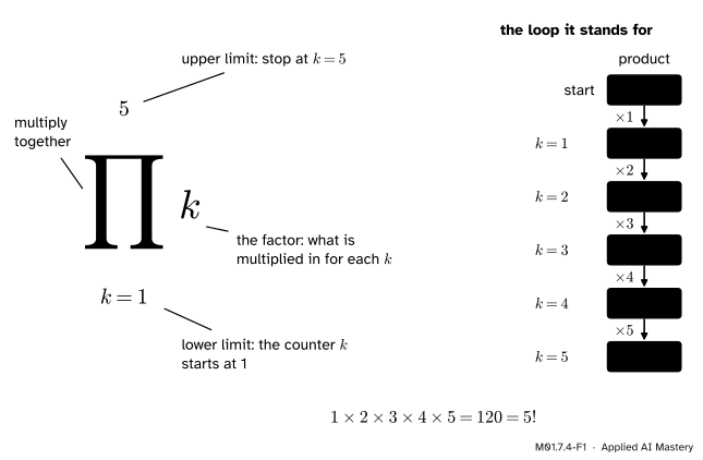
The large letter \(\prod\) is the Greek capital pi, the Greek P, for “product”. It works exactly like the sigma of M01.7.2, with multiplying in place of adding: the same counter, the same limits, the same term written beside it. The one real change is where the loop starts.
M01.7.4-F1
A product sign is a loop that multiplies. The running product starts at 1, and each value of the counter multiplies one factor in. When the counter passes the upper limit the product is done.
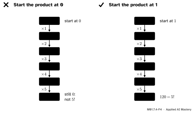
A running total starts at 0 because adding 0 changes nothing. A running product starts at 1 because multiplying by 1 changes nothing. Start a product at 0 instead and it stays 0 for ever.
as “the product of \(k\) for \(k\) from 1 to 5”. The index, the limits and the term mean what they meant for the sigma.
Step 2. Factorial. The product of the whole numbers from 1 to \(n\) is called \(n\) factorial and written \(n!\). So \({5! = 120}\), and
\[
n! = \prod_{k=1}^{n} k .
\]
Peeling off the last factor gives \({n! = n \times (n - 1)!}\), for example \({5! = 5 \times 24}\). Factorials grow fast, and M01.8.2 counts arrangements with them.
Step 3. Sums and products of nothing. A loop whose upper limit is below its lower limit, such as \(k\) from 1 to 0, never runs. It hands back its starting value. So an empty sum is 0 and an empty product is 1. These are not arbitrary choices. The step rule of a running total, \({S_n = S_{n-1} + a_n}\), must also work at \({n = 1}\), and \({S_1 = a_1}\) forces \({S_0 = 0}\). The step rule of a running product, \({P_n = P_{n-1} \times a_n}\), gives \({a_1 = P_0 \times a_1}\) at \({n = 1}\), which forces \({P_0 = 1}\).
The same reason gives \({0! = 1}\). The rule \({n! = n \times (n - 1)!}\) at \({n = 1}\) says \({1 = 1 \times 0!}\), so \(0!\) must be 1, the product of no numbers. And \({x^0 = 1}\) (M01.4.1) is the product of no copies of \(x\).
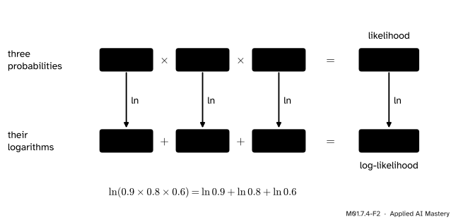
Step 4. The logarithm turns a product into a sum. For positive numbers, \({\ln(ab) = \ln a + \ln b}\) (M01.4.3). Used once per factor, the rule turns a whole product into a sum.
M01.7.4-F2
Three probabilities that a model gave to the labels it should predict. Multiplied, they give the likelihood 0.432. Their logarithms add to \({-0.8393}\), the log-likelihood, which is \(\ln 0.432\). Both routes reach the same number.
Step 5. Sums over a table. A table of numbers with rows \(i\) and columns \(j\) has the entry \(a_{ij}\) in row \(i\) and column \(j\). To add every entry you can add along each row and then add the row totals, or add down each column and then add the column totals. The worked example does both.
The formal statement
NoteDefinition: product sign, factorial, empty sum and product
If \({n < m}\), the sum \({\sum_{i=m}^{n} a_i}\) is 0 and the product \({\prod_{i=m}^{n} a_i}\) is 1. For \({n \ge 1}\), \({n! = \prod_{k=1}^{n} k}\), and \({0! = 1}\).
After \({n - 1}\) peels one factor is left, and its logarithm is the last term. Induction (M01.6.4) turns “and so on” into a proof, as in M01.7.1. The empty case agrees too: \({\ln 1 = 0}\), so the logarithm of the empty product is the empty sum. Every factor must be positive, because the logarithm of 0 or of a negative number does not exist.
Reading it. The inner sum is done first. On the left, for each row \(i\) the inner sum adds along that row, and the outer sum adds the \(m\) row totals. On the right, the inner sum adds down column \(j\), and the outer sum adds the \(n\) column totals.
Derivation. Both sides add each of the \({m \times n}\) entries exactly once. They group the entries differently, by rows or by columns. Addition does not depend on order or grouping (the commutative and associative laws of M01.1.2), so the totals agree. With finitely many terms this is only a re-ordering of one long finite sum. With infinitely many terms, re-ordering needs more care, a story for later courses.
Go deeper: the square of a sum is a double sum
Multiplying two sums means multiplying every term of the first by every term of the second, and those products fill a table:
For \({x = 1, 2, 3, 4}\) this is the 10 by 10 square of the pitfalls of M01.7.2. Its total is 100. The diagonal entries, where \({j = i}\), add to \({\sum x_i^2 = 30}\), and the other twelve, the cross terms, add to 70. That is why the square of a sum is not the sum of the squares.
Worked example
The hook’s underflow. With \({p_i = 0.1}\) for all 400 examples, the product is
The smallest positive number a standard computer float can hold is about \({5 \times 10^{-324}}\), so \({10^{-400}}\) is stored as 0.0. The sum of the logarithms is
a constant added 400 times (rule 3 of M01.7.2), and an ordinary number.
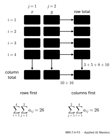
A table added two ways. Put the course’s data in a table with one row per example: row \(i\) holds \(x_i\) in column 1 and \(y_i\) in column 2, so \({a_{i1} = x_i}\) and \({a_{i2} = y_i}\).
M01.7.4-F3
Rows first: \({3 + 5 + 8 + 10 = 26}\). Columns first: \({10 + 16 = 26}\). Both routes end in the same corner, because both add every entry once.
By rows, the inner sums are \({1 + 2 = 3}\), \({2 + 3 = 5}\), \({3 + 5 = 8}\) and \({4 + 6 = 10}\), and the outer sum is 26. By columns, the inner sums are \({\sum x_i = 10}\) and \({\sum y_i = 16}\), and the outer sum is again 26. The column totals divided by 4 are the means 2.5 and 4: the mean point of the data.
Code
A product by loop, started at 1, and a factorial the same way.
# three probabilitiesp = [0.9, 0.8, 0.6]# a product starts at 1product =1# each value in turnfor value in p: product = product * valueprint("product:", round(product, 4))fact =1# k = 1, 2, 3, 4, 5for k inrange(1, 6): fact = fact * kprint("5 factorial:", fact)
product: 0.432
5 factorial: 120
A loop over an empty list never runs, so it hands back its starting values: 0 for a sum, 1 for a product.
empty_sum, empty_product =0, 1# nothing to loop overfor value in []: empty_sum = empty_sum + value empty_product = empty_product * valueprint("empty sum:", empty_sum)print("empty product:", empty_product)
empty sum: 0
empty product: 1
Now the logarithms. In Python math.log with one argument is the natural logarithm, \(\ln\). Machine-learning papers usually write this logarithm as plain “log”.
import mathlog_sum =0for value in p:# math.log(value) is ln log_sum = log_sum + math.log(value)print("sum of the logs:", round(log_sum, 4))print("log of the product:", round(math.log(product), 4))tiny =1for i inrange(400):# 400 probabilities of 0.1 tiny = tiny *0.1print("product of 400:", tiny)print("sum of logs:", round(400* math.log(0.1), 4))
sum of the logs: -0.8393
log of the product: -0.8393
product of 400: 0.0
sum of logs: -921.034
The table, added by rows and by columns with two loops, one inside the other.
# row i holds x_i and y_itable = [[1, 2], [2, 3], [3, 5], [4, 6]]by_rows =0# for each row...for row in table: row_total =0# ...add along the rowfor entry in row: row_total = row_total + entry by_rows = by_rows + row_totalby_columns =0# for each column...for j inrange(2): column_total =0# ...add down the columnfor i inrange(4): column_total = column_total + table[i][j] by_columns = by_columns + column_totalprint("rows first:", by_rows)print("columns first:", by_columns)
rows first: 26
columns first: 26
table[i][j] is the entry in row i and column j, both counted from 0. Last, the library calls.
import numpy as npprint(round(math.prod(p), 4), math.prod([]))print(math.factorial(5), math.factorial(0))t = np.array(table)print("numpy.prod:", round(np.prod(p), 4))print("axis=0, per column:", np.sum(t, axis=0))print("axis=1, per row:", np.sum(t, axis=1))print("everything:", np.sum(t))
math.prod of an empty list is 1, the empty product. With axis=0, NumPy adds down each column, across the rows, leaving one total per column. With axis=1 it adds along each row, leaving one total per row.
Explore
This module’s interactive, the sum builder, lives in lesson M01.7.3. Set its number of terms to 1 and then count up: each new bar is one more pass of the loop, added to a total that started at 0.
Pitfalls
M01.7.4-F4
Wrong beside right. A running product that starts at 0 is stuck at 0, whatever it multiplies. Started at 1, the same loop builds \({5! = 120}\).
“A running product starts at 0, like a running total.”
Then every product is 0. A total starts at 0 because adding 0 changes nothing; a product starts at 1 because multiplying by 1 changes nothing. In code, write product = 1 before the loop.
“0! is 0, because there is nothing to multiply.”
A product of nothing is 1, not 0. The rule \({n! = n \times (n - 1)!}\) at \({n = 1}\) reads \({1 = 1 \times 0!}\), which forces \({0! = 1}\). If \(0!\) were 0, the rule would give \({1! = 0}\).
“The logarithm of a sum is the sum of the logarithms.”
The rule is for products only. For example \({\ln(1 + 1) = \ln 2 \approx 0.6931}\), while \({\ln 1 + \ln 1 = 0}\). A log-likelihood is a sum of logarithms because a likelihood is a product.
“A probability of 0 does no harm.”
One factor of 0 makes the whole likelihood 0, and its logarithm does not exist: math.log(0) stops with an error. A model that is certain and wrong earns the worst possible score. The sigmoid of ML01.6 gives probabilities strictly between 0 and 1, so their logarithms always exist.
Check yourself
Recall
1. What is \({\prod_{k=1}^{4} k}\)?
Show answer
\({1 \times 2 \times 3 \times 4 = 24}\), which is \(4!\).
2. Why is a product of no numbers 1 and not 0?
Show answer
A running product starts at 1, because multiplying by 1 changes nothing, and with no factors the loop never runs. Equally, \({P_1 = P_0 \times a_1}\) must equal \(a_1\), which forces \({P_0 = 1}\).
3. What is \(0!\), and why?
Show answer
\({0! = 1}\). It is the empty product, and the rule \({n! = n \times (n - 1)!}\) at \({n = 1}\) requires it.
4. Write \(\ln(p_1 p_2 p_3)\) as a sum.
Show answer
\({\ln p_1 + \ln p_2 + \ln p_3}\), which is \({\sum_{i=1}^{3} \ln p_i}\), for positive \(p_i\).
5. Why do the row totals and the column totals of a table always add to the same number?
Show answer
Both add every entry of the table exactly once, only in a different grouping, and the order and grouping of an addition do not change its total.
Exercises
1.★ Evaluate \({\prod_{k=1}^{4} (k + 1)}\) and \({\prod_{k=1}^{3} 2}\).
a constant multiplied in \(n\) times is the constant to the power \(n\), as a constant added \(n\) times is \(n\) times the constant.
2.★★ A model gives four labels the probabilities 0.5, 0.8, 0.9 and 0.25. Find the likelihood and the log-likelihood, and check that the log-likelihood is the sum of the four logarithms.
3.★★★ The cells of a staircase have row \(i\) holding \(i\) cells, for \({i = 1, 2, 3}\). The number of cells is
\[
\sum_{i=1}^{3} \sum_{j=1}^{i} 1 .
\]
Find it by rows. Then describe the same cells column by column, write the sum with the two signs swapped, and check that it gives the same count.
Show solution
By rows: row \(i\) holds \(i\) cells, so the count is \({1 + 2 + 3 = 6}\), which is the sum of the first three whole numbers from M01.7.3.
By columns: column \(j\) holds a cell in every row \(i\) from \(j\) up to 3, which is \({3 - j + 1}\) cells. Swapping the signs must therefore change the limits, not just their order:
When the inner limits depend on the outer index, the table is a triangle, not a rectangle, and the limits must be rewritten to describe the same cells.
Summary card
A product sign is a loop that multiplies, starting at 1.
Nothing at all. An empty sum is 0, an empty product is 1, and \({0! = 1}\).
Logarithms.\({\ln \prod a_i = \sum \ln a_i}\): likelihood to log-likelihood.
Tables. Rows first or columns first, a finite double sum has the same total.
Sources and next steps
Sources. Each was opened and checked against this lesson on 12 November 2026.
Richard Hammack, Book of Proof, third edition, Section 3.4, Definition 3.1: \({0! = 1}\), with the warning that students are tempted to say \({0! = 0}\), and equation 3.1, \({n! = n \times (n - 1)!}\), which at \({n = 1}\) would give \({1! = 0}\) if \(0!\) were 0.
Ian Goodfellow, Yoshua Bengio and Aaron Courville, Deep Learning, Chapter 5, Section 5.5: the likelihood as a product over the examples (equation 5.57), the remark that such a product is prone to numerical underflow, and the logarithm that turns it into a sum (equation 5.58).
Eric Lehman, F. Thomson Leighton and Albert R. Meyer, Mathematics for Computer Science (MIT 6.042J, revised May 2015), Section 13.6: a double sum over a triangle of pairs, added row by row or column by column, with the limits rewritten when the order is swapped.
Python 3.12 documentation, math.prod and math.factorial: prod starts from 1 and returns that start value for an empty list. NumPy reference, numpy.prod and numpy.sum: the product of an empty array is the neutral element 1, the sum of an empty array is 0, and the axis argument chooses the direction of the sum.
Next. Module M01.8 Counting and combinatorics puts factorials to work counting arrangements. Logarithms of products return in ML01.6, as the log loss.