The capital Greek letter sigma writes a long sum as one symbol, and it reads as a loop: a counter, where it starts and stops, and the term to add. Expand and fold sums, rename the counter, derive three rules, and write the mean, the mean squared error and a distance with it.
Read a sum written with a sigma aloud, naming its index, its lower and upper limits and its term, and count its terms.
Expand a sigma into its terms and fold a written-out sum back into a sigma, renaming or shifting the index where that helps.
Derive the constant-factor, sum-of-sums and constant-term rules by writing out the terms, and use them to simplify a sum.
Write the mean, the mean squared error and the distance between two points as sigma expressions and evaluate them on the course’s data.
Compute a sum with a loop that keeps a running total, then with sum, numpy.sum and numpy.mean.
In review. The maths and code on this page are checked by automated tests on every change, but an independent reader has not signed it off yet. Spot a mistake or a confusing step? Tell us.
The question
Open almost any machine-learning text and one of the first formulas is the loss of a model. For a model that predicts \(\hat{y}_i\) where the target is \(y_i\), on \(n\) examples, it is written
One Greek letter stands in for a whole loop over the data. What exactly does it tell you to do, and how can you work with it without writing out every term?
From the last lesson
1. What is the 20th term of 2, 5, 8, 11, and so on?
Show answer
\({a_{20} = 2 + 19 \times 3 = 59}\).
2. Which term of the doubling sequence 1, 2, 4, 8 is 1024?
Show answer
The 11th. The terms are \({a_n = 2^{\,n-1}}\) and \({1024 = 2^{10}}\), so \({n - 1 = 10}\).
Intuition
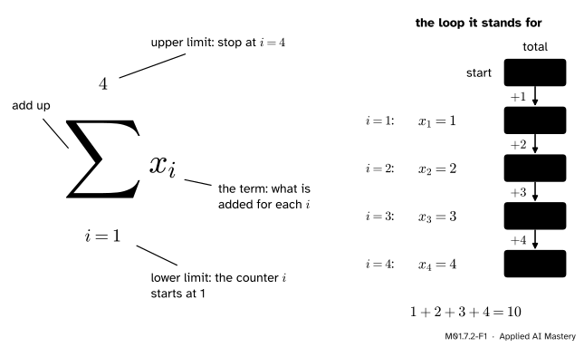
The large letter \(\sum\) is the Greek capital sigma, the Greek S, for “sum”. It is an instruction to add things up, and the small writing around it says exactly what to add. Below it sits a counter and where it starts. Above it sits where the counter stops. To its right sits the thing to add for each value of the counter. The figure names each part and runs the loop it stands for, on the course’s four inputs \(x_1\) to \(x_4\), which are 1, 2, 3 and 4.
M01.7.2-F1
A sigma is a loop. The total starts at 0. The counter \(i\) takes the values 1, 2, 3, 4 in turn, and for each value the term \(x_i\) is added on. When the counter passes the upper limit, the loop stops and the total is the value of the sum.
Read the expression aloud as “the sum of \(x_i\) for \(i\) from 1 to 4”. In Python it is a loop that keeps a running total, and the code section writes exactly that loop.
Build it up
Step 1. The parts. In
\[
\sum_{i=1}^{4} x_i
\]
the letter \(i\) is the index, a counter. The lower limit 1 is where it starts, the upper limit 4 is where it stops, and \(x_i\) is the term: what gets added for each value of \(i\). The limits are both included, so a sum from 1 to 4 has 4 terms and a sum from 3 to 7 has \({7 - 3 + 1 = 5}\) terms.
Step 2. Writing a sum out. Put each value of the index into the term in turn, and add:
Step 3. Folding a sum back. Going the other way, look for what changes from term to term. In \({3 + 6 + 9 + \dots + 30}\) the \(k\)-th term is \(3k\), and the last one, 30, is \({3 \times 10}\), so
Step 4. The index’s name does not matter. The sums \({\sum_{i=1}^{4} x_i}\) and \({\sum_{j=1}^{4} x_j}\) give the same instructions and the same total. The index is a placeholder, like the name of the loop variable in code.
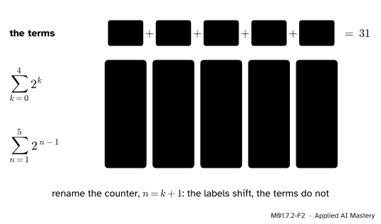
Step 5. Shifting the index. The doubling numbers \({1 + 2 + 4 + 8 + 16}\) can be counted from 0, with term \(2^k\), or from 1, with term \({2^{\,n-1}}\).
M01.7.2-F2
One sum, two labellings. Setting \({n = k + 1}\) moves both limits up by 1 and replaces \(k\) by \({n - 1}\) in the term. The five terms, and their total 31, do not change.
So shifting is safe as long as you change the limits and the term together.
Why. Write out the left side, take off the brackets, and move every \(b\) to the back. Adding in a different order or grouping gives the same total (the commutative and associative laws):
There is no such rule for products or squares. The pitfalls below show why.
Worked example
The course’s data are the four points with \({x = 1, 2, 3, 4}\) and \({y = 2, 3, 5, 6}\), and the line \({\hat{y} = 1.4x + 0.5}\), taken as given here (ML01.4 derives it).
The mean. The mean of \(x\) is the sum divided by how many there are:
In the same way \({\bar{y} = (2 + 3 + 5 + 6)/4 = 4}\), so the mean point is \((2.5, 4)\), as in M01.2.1.
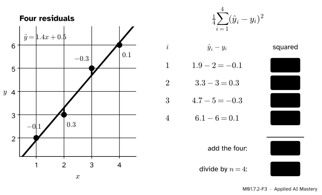
The mean squared error. The line’s predictions are \({\hat{y}_i = 1.4x_i + 0.5}\), which gives 1.9, 3.3, 4.7 and 6.1. Each term of the loss is one error, squared.
M01.7.2-F3
The sigma, one term per point. Each error is a prediction minus a target. Squared, the four errors are 0.01, 0.09, 0.09 and 0.01. They add to 0.2, and dividing by 4 gives 0.05.
For \({P = (1, 2)}\) and \({Q = (4, 6)}\) the sum is \({3^2 + 4^2 = 25}\), and \({\sqrt{25} = 5}\). In space, from \((1, 2, 3)\) to \((2, 4, 5)\), the sum is \({1 + 4 + 4 = 9}\), and \({\sqrt{9} = 3}\). The square root sits outside the sigma: add every squared change first, then take one root.
Code
A sigma is a loop that keeps a running total. Here it is for the sum and the mean of \(x\).
# the inputs x_1 to x_4x = [1, 2, 3, 4]# the targets y_1 to y_4y = [2, 3, 5, 6]# the running totaltotal =0# i takes the values 0, 1, 2, 3for i inrange(len(x)):# add the term for i total = total + x[i]print("sum of x:", total)print("mean of x:", total /len(x))
sum of x: 10
mean of x: 2.5
Python’s index runs from 0 to 3, so x[i] covers \(x_1\) to \(x_4\) of the maths. The mean squared error is the same loop with a different term.
# the course's linew, b =1.4, 0.5# running total of squaressquares =0for i inrange(len(x)):# prediction for example i y_hat = w * x[i] + b squares = squares + (y_hat - y[i]) **2mse = squares /len(x)print("sum of squared errors:", round(squares, 4))print("mean squared error:", round(mse, 4))
sum of squared errors: 0.2
mean squared error: 0.05
The total prints as 0.2 after rounding. Unrounded it is a hair off, because a computer stores a number such as 1.4 only approximately (M01.1.1). The distance is one more loop, then a square root.
import mathP, Q = (1, 2), (4, 6)squares =0# one pass per coordinatefor i inrange(len(P)): squares = squares + (Q[i] - P[i]) **2print("by the sigma:", math.sqrt(squares))print("by math.dist:", math.dist(P, Q))
by the sigma: 5.0
by math.dist: 5.0
Now the library versions. Python’s sum adds a list for you, and NumPy adds a whole array, or averages it, in one call. The last line is the hook’s formula: the loss in a single line.
This module’s interactive, the sum builder, lives in lesson M01.7.3. It writes every sum it builds three ways at once: as a sigma, as its terms written out, and as one number.
Pitfalls
M01.7.2-F4
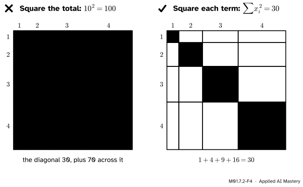
Wrong beside right, when the goal is \(\sum x_i^2\). Squaring the total counts the whole 10 by 10 square, 100. Adding the squares counts only the four squares on the diagonal, 30.
“The sum of the squares is the square of the sum.”
For \({x = 1, 2, 3, 4}\), the sum of the squares is \({1 + 4 + 9 + 16 = 30}\), but the square of the sum is \({10^2 = 100}\). Squaring the total also counts every product of two different terms, the off-diagonal blocks of the figure, which add to 70. Formulas for spread, such as the variance of S01.3, depend on keeping these two apart.
Rule 1 moves a factor outside only when it is the same in every term, and \(y_i\) changes with \(i\).
“Adding a constant gives the constant.”
A term with no index in it is still added once for each value of the index. So \({\sum_{i=1}^{4} 0.5 = 4 \times 0.5 = 2}\), not 0.5.
“Python’s range(1, n) runs up to n.”
It stops one short. range(1, 4) gives 1, 2, 3, while the sigma from 1 to 4 includes 4. To run over positions 1 to \(n\), write range(1, n + 1), or loop over indices 0 to \({n - 1}\) with range(n) and remember that index \(i\) holds term \({i + 1}\).
Check yourself
Recall
1. Read \({\sum_{i=1}^{4} x_i}\) aloud, and name its four parts.
Show answer
“The sum of \(x_i\) for \(i\) from 1 to 4.” The index is \(i\), the lower limit 1, the upper limit 4, and the term \(x_i\).
2. How many terms does \({\sum_{k=3}^{7} a_k}\) have?
Show answer
Five: \({7 - 3 + 1 = 5}\). They are \(a_3, a_4, a_5, a_6\) and \(a_7\).
3. Write \({1 + 4 + 9 + 16 + 25}\) with a sigma.
Show answer
\({\sum_{k=1}^{5} k^2}\), which is 55.
4. What is \({\sum_{i=1}^{10} 3}\)?
Show answer
\({10 \times 3 = 30}\): the term 3 is added once for each of the ten values of \(i\).
5. Write the mean squared error of predictions \(\hat{y}_i\) against targets \(y_i\), over \(n\) examples, with a sigma.
Show answer
\[
L = \frac{1}{n} \sum_{i=1}^{n} (\hat{y}_i - y_i)^2 .
\]
Exercises
1.★ Write out and evaluate \({\sum_{k=1}^{4} (2k + 1)}\). Then get the same answer from the three rules.
Show solution
Written out: \({3 + 5 + 7 + 9 = 24}\). By the rules, split the sum (rule 2), take out the 2 (rule 1) and add the constant 1 four times (rule 3):
2.★★ For the course’s inputs, \({\sum x_i = 10}\) and \({\sum x_i^2 = 30}\), with \(i\) from 1 to 4. Use only these two totals and the rules to find \({\sum_{i=1}^{4} (x_i - 2.5)^2}\), then check it term by term.
Term by term, the four squares 2.25, 0.25, 0.25 and 2.25 add to 5. This is the total squared distance of the inputs from their mean, the start of the variance.
3.★★★ Without using the four errors themselves, show that the errors \({\hat{y}_i - y_i}\) of the line \({\hat{y} = 1.4x + 0.5}\) on the course’s data add to zero. Then say why the loss squares the errors before adding them.
Show solution
Split the sum (rule 2, for a difference), then split \({\hat{y}_i = 1.4x_i + 0.5}\) the same way and use rules 1 and 3:
The errors \({-0.1, 0.3, -0.3, 0.1}\) do add to 0. A loss that added raw errors would call this line perfect, and would also call perfect a line with errors of \({-5}\) and \({+5}\). Squaring makes every error count as positive, so errors cannot cancel.
Summary card
A sigma is a loop that adds: a counter, its start and stop, and a term.
M01.7.2-F1
Start at 0; add one term per value of the index.
Definition.\({\sum_{i=m}^{n} a_i = a_m + \dots + a_n}\), with \({n - m + 1}\) terms.
Rules. Constants come outside; sums split; \({\sum_{i=1}^{n} c = n\,c}\).
No such rule for squares or products: \({\sum x_i^2 \ne \big(\sum x_i\big)^2}\).
Mean squared error.\({\frac{1}{n}\sum_{i=1}^{n} (\hat{y}_i - y_i)^2}\), which is 0.05 here.
Sources and next steps
Sources. Each was opened and checked against this lesson on 12 November 2026.
Jay Abramson and others, Algebra and Trigonometry, 2nd edition (OpenStax), Section 13.4, under “Using Summation Notation”: it calls \(k\) the index of summation, 1 the lower limit of summation and \(n\) the upper limit of summation.
Ian Goodfellow, Yoshua Bengio and Aaron Courville, Deep Learning, Chapter 5, Section 5.1.4, equation 5.4, writes the mean squared error on a test set as \(\frac{1}{m}\) times a sum over the examples of the squared differences between predictions and targets.
Python 3.12 documentation, the built-in function sum, which adds a start value, 0 by default, and the items of a list from left to right; and the NumPy reference, numpy.sum.