On a log scale every equal step multiplies by the same factor, so one ruler can show 0.0001 and 1,000,000 together. Learn to read log axes and orders of magnitude, and see why machine learning adds logarithms instead of multiplying probabilities.
Place numbers on a log scale, and read values, including halfway points, from a log axis.
State the order of magnitude of a number and compare two numbers by their ratio.
Recognise exponential growth or decay as a straight line on a log axis.
Explain why a long product of probabilities underflows in floating point while the sum of their logarithms does not, and compute minus the logarithm of a probability.
In review. The maths and code on this page are checked by automated tests on every change, but an independent reader has not signed it off yet. Spot a mistake or a confusing step? Tell us.
The question
People tuning a model try the learning rates 0.0001, 0.001, 0.01 and 0.1. On an ordinary axis from 0 to 0.1 the first three are squeezed into its first tenth, and the first two land almost on top of each other. Then a model multiplies 400 probabilities of 0.1, and Python reports that the product is exactly 0.0. What do these two problems have in common, and what cures both?
From the last lesson
1. What are \(\log_{10} 1\), \(\log_{10} 10\) and \(\log_{10} 0.01\)?
Show answer
0, 1 and \({-2}\), because \({10^0 = 1}\), \({10^1 = 10}\) and \({10^{-2} = 0.01}\).
2. State the product law of logarithms and the rule of powers it comes from.
Show answer
\({\log_b(uv) = \log_b u + \log_b v}\). It comes from the product rule \({b^m\, b^n = b^{m+n}}\).
Intuition
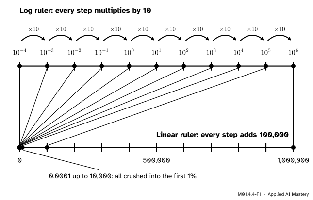
A ruler puts each number at some distance from its start. On an ordinary, linear ruler, equal distances mean equal differences: on a ruler from 0 to 1,000,000, every tenth of its length adds 100,000. Now mark on it the eleven numbers 0.0001, 0.001, 0.01 and so on up to 1,000,000, each ten times the one before. Nine of them land in the first 1% of the ruler. Only 100,000 and 1,000,000 can be told apart.
On a log ruler a number sits at its logarithm: \(10^k\) sits at position \(k\). Now equal distances mean equal ratios, because every step multiplies by 10, and the same eleven numbers sit at eleven evenly spaced marks.
M01.4.4-F1
The same eleven values on two rulers. On the linear ruler they crowd into the first 1%; on the log ruler each one is a single step from the next, and every step multiplies by 10.
This is the ladder of M01.4.1 once more: the exponents are evenly spaced, and the values they stand for multiply as you go. A log ruler lets the eye compare 0.0001 with 1,000,000, which no linear ruler can do.
Build it up
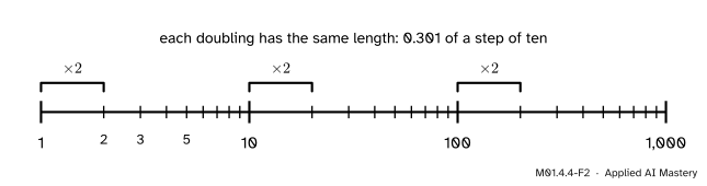
Step 1. Positions between the powers of ten. On a log ruler with base 10, the number \(x\) sits at position \(\log_{10} x\), measured in steps of ten called decades. So 1 is at 0, 10 at 1, 100 at 2 and 0.1 at \({-1}\). The numbers in between sit at their logarithms too: 2 at about 0.301, 3 at 0.477 and 5 at 0.699. The marks 2, 3, …, 9 therefore crowd towards 10.
M01.4.4-F2
Reading a log axis. The ticks of each decade bunch up towards the next power of ten, and every doubling has the same length, wherever it starts.
Step 2. Equal ratios, equal lengths. From 1 to 2, from 10 to 20 and from 100 to 200 are the same length, 0.301 of a decade, because each is a doubling. By the quotient law of M01.4.3:
\[
\log_{10} 20 - \log_{10} 10 = \log_{10} 2 .
\]
Step 3. Orders of magnitude. The order of magnitude of a positive number is its position on the log ruler rounded down: the exponent of the power of ten at or just below it. In the scientific notation \({a \times 10^n}\) of M01.4.1, it is \(n\). So 3,500 has order of magnitude 3 and 0.0003 has order of magnitude \({-4}\). One number is \(k\) orders of magnitude above another when it is about \(10^k\) times as big: 1,000,000 is ten orders of magnitude above 0.0001.
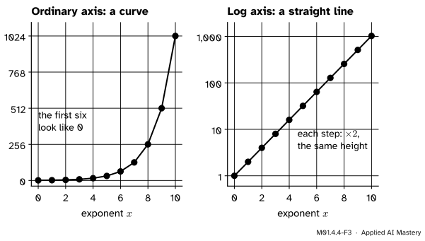
Step 4. Log axes. A plot can use a log ruler as an axis. Then a quantity that is multiplied by the same factor at every step climbs the same height at every step, so its points lie on a straight line.
M01.4.4-F3
The doubling sequence on an ordinary axis and on a log axis. Multiplying by 2 at every step bends the first picture and straightens the second.
In machine learning, a search for a good learning rate typically tries values spaced evenly on a log scale, such as 0.1, 0.01, 0.001 and 0.0001, so that each size gets a fair look, and plots the results against a log axis. A loss that falls from 1 to 0.001 is easier to follow on a log axis too, because each factor of 10 takes the same height.
The formal statement
NoteDefinition: log scale
On a log scale with base 10, a number \({v > 0}\) sits at position \(\log_{10} v\). A log axis is an axis of a plot drawn as a log scale.
Four results follow from the laws of M01.4.3.
Result 1: distance measures the ratio. By the quotient law, the distance from \(u\) to \(v\) is
\[
\log_{10} v - \log_{10} u = \log_{10} \frac{v}{u} .
\]
It depends only on the ratio \(v / u\). Equal ratios give equal distances: every factor of 10 is one decade long, every factor of 2 is 0.301 decades.
Result 2: halfway is the square root of the product. The point halfway between \(u\) and \(v\) sits at the average of their positions. The product law and then the power law with \({k = \frac12}\) give
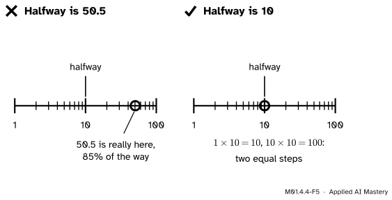
So halfway between 1 and 100 on a log axis is \({\sqrt{100} = 10}\), not 50.5.
Result 3: exponentials are straight lines. For \({f(x) = a\, b^x}\) with \({a > 0}\), the product law and then the power law give
\[
\begin{aligned}
\log_{10} f(x) &= \log_{10} a + \log_{10}\left(b^x\right) \\
&= \log_{10} a + x \log_{10} b .
\end{aligned}
\]
That is a line in \(x\) with slope \(\log_{10} b\), so on a log axis the graph of an exponential is straight. Growth climbs and decay falls.
Result 4: a product becomes a sum. The product law splits off one factor at a time, so the logarithm of a product of any number of factors is the sum of their logarithms. For three:
(M01.7.4 writes this for any number of factors with a single sign.)
Why machine learning takes logs. A model that predicts probabilities is judged by the probability it gave to everything that really happened, and for separate examples those probabilities multiply (ML01.6.2 calls the product the likelihood). With hundreds of examples or more, that product is far too small for a computer. A Python float holds positive numbers with full precision down to about \({2.2 \times 10^{-308}}\) and, with fewer digits, down to about \({5 \times 10^{-324}}\). A result below about half of that is rounded to 0.0. This is called underflow.
The logarithm is the cure. By Result 4 the logarithm of the product is a sum of ordinary-sized numbers, which never underflows. And because \(\ln\) increases (its graph only climbs), a bigger product always has a bigger logarithm, so comparing sums of logarithms picks the same best model as comparing the products would.
The logarithms of probabilities are negative, since \({\ln p < 0}\) whenever \({0 < p < 1}\). So it is usual to work with \({-\ln p}\), which is 0 when the model was certain and right (\({p = 1}\)) and grows without limit as \(p\) shrinks: \({-\ln 0.9 \approx 0.1054}\), \({-\ln 0.5 \approx 0.6931}\) and \({-\ln 0.1 \approx 2.3026}\). Its average over the examples is the log loss, the main subject of ML01.6.2.
Worked example
Multiply 400 probabilities of 0.1, and then add their logarithms instead.
By hand. Since \({0.1 = 10^{-1}}\), the power-of-a-power rule gives the product at once:
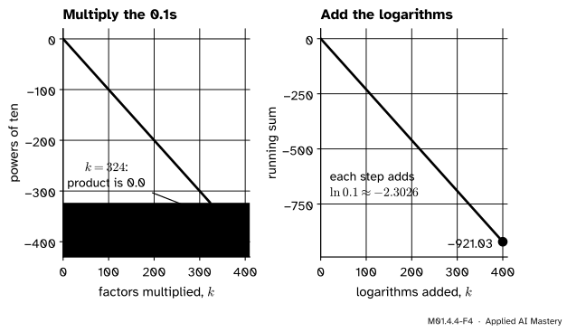
In the computer. The true product, \({10^{-400}}\), is about 77 orders of magnitude below the smallest positive float, which is about \({10^{-323.3}}\). Multiplying in one factor at a time, the running product shrinks by a factor of 10 at each step. Below \({10^{-308}}\) it starts to lose digits, and at the 324th factor it becomes exactly 0.0. From then on it stays 0.0, whatever comes next, and its logarithm does not exist.
M01.4.4-F4
The worked example as a trace. Left: multiplied one factor at a time, the product falls off the bottom of the floats and becomes 0.0 at the 324th factor. Right: the sum of the logarithms falls steadily to \({-921.03}\), and nothing is lost.
Adding logarithms instead. Each factor contributes \({\ln 0.1 \approx -2.3026}\), so after 400 factors the running sum is \({-921.03}\): an ordinary number that a float holds with ease. And each example’s \({-\ln p}\) is 2.3026, so the log loss of a model that gives every right answer a probability of 0.1 is 2.3026.
Code
Both computations by loop. The first multiplies, and records the first factor after which nothing is left:
probs = [0.1] *400# a list of 400 copies of 0.1product =1.0first_zero =Nonefor k, p inenumerate(probs, start=1): # k counts the factors from 1 product = product * pif product ==0.0and first_zero isNone: first_zero = k # the first factor that left nothingprint(product, first_zero) # 0.0 324
0.0 324
The second adds the natural logarithms instead:
import mathtotal =0.0for p in probs: total = total + math.log(p) # add ln p instead of multiplying by pprint(round(total, 2)) # -921.03print(round(400* math.log(0.1), 2)) # the power law in one line: -921.03print(math.ulp(0.0)) # the smallest positive float: 5e-324for p in [0.9, 0.5, 0.1]:print(p, round(-math.log(p), 4)) # minus ln p: 0.1054, 0.6931, 2.3026
NumPy does each in one line, and numpy.logspace makes a grid of learning rates that is even on a log scale: four values from \({10^{-4}}\) to \({10^{-1}}\), one per decade.
import numpy as npprobs_array = np.full(400, 0.1) # the same 400 probabilities, as an arrayprint(np.prod(probs_array)) # 0.0: the product underflowsprint(round(np.log(probs_array).sum(), 2)) # -921.03: the sum of the logs does notlearning_rates = np.logspace(-4, -1, 4) # 10 to the -4, -3, -2 and -1print(learning_rates)print(np.log10(learning_rates)) # equal steps on a log scale
To see the results of such a grid, plot the loss against the learning rate and switch the horizontal axis to a log scale. This is the Matplotlib call, shown here but not run (lessons do not draw plots; final_losses would come from your own training runs):
import matplotlib.pyplot as pltfig, ax = plt.subplots()ax.plot(learning_rates, final_losses, marker="o")ax.set_xscale("log") # equal steps along the axis now mean equal factors
Explore
M01.4-X1
Log ruler
Slide the ruler from linear to logarithmic and watch the crowded values from 1 to 1,000,000 spread out until every step multiplies by 10. Then choose \(a\) and \(b\): their lengths laid end to end land on \({a + b}\) on the linear ruler and on \({a \times b}\) on the log ruler, as on a slide rule.
Pitfalls
M01.4.4-F5
Wrong beside right. On a log axis from 1 to 100, halfway is 10, the square root of \({1 \times 100}\). The number 50.5 sits 85% of the way along.
“Halfway along a log axis from 1 to 100 is 50.5.”
On a log axis halfway means halfway in ratio: 1 to 10 is one factor of 10, and 10 to 100 is another. By Result 2 the midpoint is \({\sqrt{1 \times 100} = 10}\). Reading a log axis as if it were linear is an easy way to misread a plot of loss or of learning rates.
“A log axis can start at 0.”
0 has no logarithm: each step to the left only divides by 10, so 0 is infinitely far away. A log axis starts at some positive number, such as \({10^{-4}}\). Values of 0 or below cannot be drawn on it; NumPy’s log returns -inf for 0 and nan for a negative number.
“The computer says the product is 0.0, so the probability is 0.”
It is underflow, not a fact about the data. The true product, \({10^{-400}}\), is tiny but positive. Never multiply long runs of probabilities in floating point; add their logarithms.
Check yourself
Recall
1. On a log ruler, which is longer: from 1 to 10, or from 1,000 to 10,000?
Show answer
Neither: both are one factor of 10, one decade, so they have the same length.
2. What is the order of magnitude of 0.0003?
Show answer
\({-4}\), since \({0.0003 = 3 \times 10^{-4}}\).
3. A quantity doubles at every step. What does its graph look like on a log axis?
Show answer
A straight line, rising by \({\log_{10} 2 \approx 0.301}\) decades at every step.
4. Why does the product of 400 probabilities of 0.1 come out as 0.0 in Python?
Show answer
The true product is \({10^{-400}}\), far below the smallest positive float (about \({5 \times 10^{-324}}\)), so it underflows and is rounded to 0.0.
5. What is \({-\ln 0.5}\), and why is \({-\ln p}\) positive whenever \({0 < p < 1}\)?
Show answer
About 0.6931. For \({0 < p < 1}\) the logarithm \(\ln p\) is negative, so \({-\ln p}\) is positive.
Exercises
1.★ On a log ruler with 1 at position 0 and one unit per decade, where do 0.01, 3 and 2,000 sit?
Show solution
At their logarithms to base 10. \({\log_{10} 0.01 = -2}\). \({\log_{10} 3 \approx 0.4771}\). And by the product law,
The first is one decade from each end. In the second, 2 to 10 and 10 to 50 are both a factor of 5.
3.★★★ A model gives the probabilities 0.9, 0.5 and 0.2 to three correct answers. (a) Find the product, and the sum of the natural logarithms, and check that \(e\) to the power of the sum is the product. (b) Find \({-\ln p}\) for each answer and their average, the log loss. (c) What would \({-\ln p}\) be for a confident wrong answer with \({p = 0.001}\)?
Show solution
(a) The product is 0.09, since 0.9 times 0.5 is 0.45 and 0.45 times 0.2 is 0.09. The logarithms are about \({-0.1054}\), \({-0.6931}\) and \({-1.6094}\), and their sum is about \({-2.4079}\). By Result 4 this is \(\ln 0.09\), so \({e^{-2.4079} \approx 0.09}\), the product.
(b) The three values of \({-\ln p}\) are 0.1054, 0.6931 and 1.6094. Add them and divide by 3:
(c) \({-\ln 0.001 \approx 6.9078}\), more than eight times the average above. Because \({-\ln p}\) grows without limit as \(p\) shrinks, one confident mistake costs more than many small doubts.
Summary card
On a log scale equal steps mean equal factors; in machine learning, logarithms turn products into sums.
M01.4.4-F1
One ruler for a millionth and a million.
\[
\ln(p_1 p_2) = \ln p_1 + \ln p_2
\]
Position of \(v\) on a log scale: \(\log_{10} v\). Distance from \(u\) to \(v\): \(\log_{10}(v/u)\).
Halfway between \(u\) and \(v\) on a log axis: \(\sqrt{uv}\).
Exponential growth or decay is a straight line on a log axis.
\(0.1^{400}\) underflows to 0.0; \({400 \ln 0.1 \approx -921.03}\) does not.
\({-\ln p}\) is the log loss of one example, ML01.6.
Sources and next steps
Sources. Each was opened and checked against this lesson on 12 November 2026.
Daniel Jurafsky and James H. Martin, Speech and Language Processing, 3rd edition draft of 19 August 2026, Chapter 3, Section 3.1.3: language model probabilities are stored and computed as log probabilities, because multiplying enough probabilities together results in numerical underflow, and adding in log space is equivalent to multiplying in linear space (Equation 3.13). The book writes log for the natural logarithm.
Python Software Foundation, math.ulp and sys.float_info, Python 3.12 documentation: math.ulp(0.0) is the smallest positive denormalised float, smaller than sys.float_info.min, the minimum positive normalised float.
NumPy, numpy.logspace (“Return numbers spaced evenly on a log scale”, from base ** start to base ** stop) and numpy.log (the natural logarithm, which returns -inf for 0 and nan for values with no real logarithm), NumPy 2.5 manual.
Matplotlib, Axes.set_xscale, Matplotlib 3.11.2 documentation: set_xscale("log") draws the horizontal axis on a log scale.
Ian Goodfellow, Yoshua Bengio and Aaron Courville, Deep Learning, MIT Press, 2016, Chapter 11, Section 11.4.3, Grid Search: a grid search typically picks values approximately on a logarithmic scale, such as a learning rate from the set 0.1, 0.01, \({10^{-3}}\), \({10^{-4}}\) and \({10^{-5}}\); its Figure 11.1 plots the training error against the learning rate on a logarithmic scale.
Next. The log loss is built in lesson ML01.6.2, The log loss, linked below. Statistics uses the logarithms of skewed data, such as rents, in S01.4.