Reading notation: subscripts, Greek letters and formulas
Read a formula aloud, symbol by symbol: variables, constants and parameters, subscripts that label the items of a list, hats for predictions and bars for means, the signs of comparison, and the Greek letters later courses use, all worked on this course’s four data points.
Read a formula such as y-hat sub i = w x sub i + b aloud, and say which of its symbols are variables, parameters and constants.
Use subscripts to name the items of a list, counting from 1 in maths and from 0 in Python.
Explain what a hat and a bar on a letter mean, and compute the predictions and the mean of a small data set by hand.
Name the twelve Greek letters that later courses use most, and say what each usually stands for.
In review. The maths and code on this page are checked by automated tests on every change, but an independent reader has not signed it off yet. Spot a mistake or a confusing step? Tell us.
The question
Here is a line from a machine-learning text: \({\hat{y}_i = w x_i + b}\). Can you read it aloud? What do the hat, the small \(i\) and the letters \(w\) and \(b\) each tell you? By the end of this lesson you will read it, and work it out for the four data points of this course, by hand and in Python.
From the last lesson
1. When does the sign of an inequality flip?
Show answer
When both sides are multiplied or divided by a negative number, because that turns the number line round.
2. Rearrange \({y = wx + b}\) to make \(x\) the subject.
Show answer
\({x = (y - b)/w}\), which needs \(w\) to be not 0.
Intuition
A formula is a sentence, and each symbol in it is a word with a job. Some symbols hold the data you were given. Some are numbers that shape the rule. Some are results worked out from the others. Once you can name each job, you can read the sentence aloud.
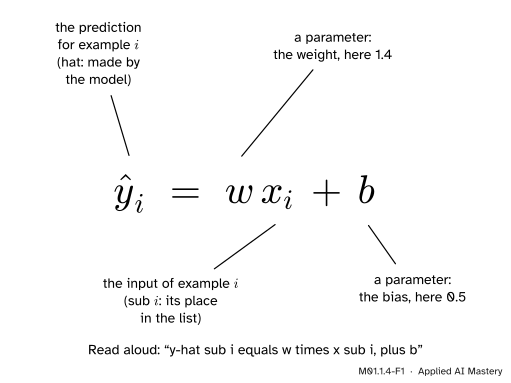
M01.1.4-F1
One formula, every part named. Blue is data given to the model, orange shapes the rule, and vermillion is the model’s output.
Read it as “y-hat sub \(i\) equals \(w\) times x sub \(i\), plus \(b\)”. In words: the prediction for example number \(i\) is its input times 1.4, plus 0.5. That is the whole sentence.
Build it up
Step 1. Three jobs for a letter. A variable changes from case to case: the input \(x\) is different for every example. A parameter is fixed while a model is used but chosen when it is built: the weight \(w\) and the bias \(b\). Learning, in machine learning, means choosing them. A constant never changes at all: 2, or \({\pi \approx 3.1416}\). The same letter can do different jobs in different texts, so a good text always says what its letters mean.
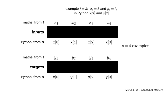
Step 2. Subscripts label the items of a list. The course’s data are four inputs and four targets. We call the inputs \(x_1, x_2, x_3, x_4\), read “x sub 1” and so on, and the targets \(y_1, \dots, y_4\). The small number is a subscript: it says which item, not how big it is.
M01.1.4-F2
Subscripts are labels on a list. Maths counts from 1; Python counts positions from 0, so \(x_3\) is x[2].
To talk about any one of them we write \(x_i\), “the \(i\)-th x”, where the index\(i\) can be 1, 2, 3 or 4. The number of items is \(n\), here \({n = 4}\), and the whole list is written \(x_1, x_2, \dots, x_n\): the dots mean “and so on, in the same pattern”. Example \(i\) is the pair \((x_i, y_i)\). In Python the same list is x[0], x[1], x[2], x[3]: position 0 holds \(x_1\).
Step 3. Hats and bars. A hat marks a value made by a model: \(\hat{y}_i\) is the prediction for example \(i\), while \(y_i\) is the true target. A bar marks a mean: \(\bar{x}\), “x-bar”, is the mean of all the \(x\)’s. Lesson M01.7.2 will write sums with a sigma; for now we write them out with dots.
Step 4. Signs of comparison.
Sign
Read as
Example
\({=}\)
equals
\({\hat{y}_3 = 4.7}\)
\({\neq}\)
is not equal to
\({\hat{y}_1 \neq y_1}\)
\({\approx}\)
is approximately equal to
\({\sqrt{2} \approx 1.4142}\)
\({<}\)
is less than
\({x_1 < x_2}\)
\({\leq}\)
is less than or equal to
\({x_i \leq 4}\)
Turned round, \({>}\) and \({\geq}\) read “is greater than” and “is greater than or equal to”.
Step 5. Greek letters. Mathematics runs out of Latin letters quickly, so it borrows Greek ones. These twelve appear again and again in the courses ahead:
Letter
Read as
Later it usually stands for
\(\alpha\)
alpha
a step size; some books call the learning rate \(\alpha\) (ML01.5)
\(\beta\)
beta
a weight that balances two scores (ML01.7)
\(\gamma\)
gamma
the discount rate of reinforcement learning (RL01)
\(\delta\)
delta
a small change (ML01.4)
\(\varepsilon\)
epsilon
a small amount, or noise in a measurement (ML01.4)
\(\eta\)
eta
the learning rate (ML01.5)
\(\theta\)
theta
an angle (M01.5), or all the parameters of a model
\(\lambda\)
lambda
the price of a penalty on large weights (ML01.9)
\(\mu\)
mu
the mean of a whole population (S01)
\(\pi\)
pi
the number 3.14159… (M01.5); a policy in RL01
\(\sigma\)
sigma
a standard deviation (S01); the sigmoid (ML01.6)
\(\phi\)
phi
the phase of a wave (M01.5)
Epsilon and phi each have a second shape, \(\epsilon\) and \(\varphi\); they are the same letters. The capital sigma, \(\Sigma\), is the sum sign of lesson M01.7.2. The site’s notation page lists every symbol the courses use.
The formal statement
NoteDefinitions: lists, predictions and the mean
A list of \(n\) numbers is written \(x_1, x_2, \dots, x_n\). Its \(i\)-th item is \(x_i\), and \(i\) is the index. In Python the same list is x[0], …, x[n - 1].
A data set of \(n\) examples is the list of pairs \((x_1, y_1), \dots, (x_n, y_n)\): an input and its target.
The model’s prediction for example \(i\) is \({\hat{y}_i = w x_i + b}\).
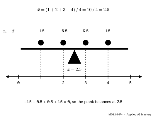
The mean has a balance property. Take the difference \({x_i - \bar{x}}\) between each item and the mean: it is negative for an item to the left of the mean and positive for one to the right. These differences always add up to 0:
The first step collects the \(x\)’s together and the \(n\) copies of \(\bar{x}\) together, which the commutative and associative laws of lesson M01.1.2 allow. The next step uses the definition of the mean, multiplied through by \(n\): \({x_1 + x_2 + \dots + x_n = n\,\bar{x}}\).
M01.1.4-F4
The mean is the balance point. Equal weights at 1, 2, 3 and 4 balance on a wedge at \({\bar{x} = 2.5}\), because their differences from 2.5 add up to 0.
Worked example
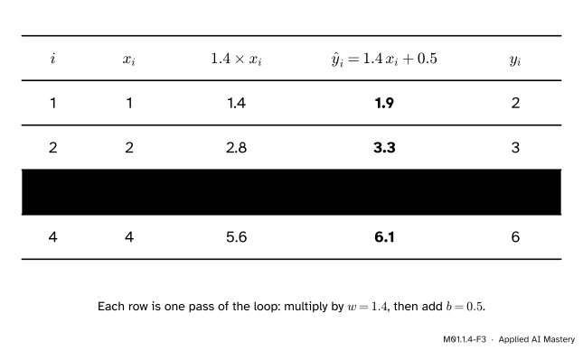
The course’s data are the inputs 1, 2, 3, 4 with the targets 2, 3, 5, 6. The model is \({\hat{y}_i = 1.4 x_i + 0.5}\), taken as given here (lesson ML01.4 shows where it comes from). Compute every prediction, and the means \(\bar{x}\) and \(\bar{y}\).
M01.1.4-F3
The predictions as a trace, one row per example. Each row multiplies by the weight and then adds the bias, in the order of lesson M01.1.2.
Put \({i = 1, 2, 3, 4}\) into the formula in turn:
Compare each with its target. \({\hat{y}_1 = 1.9}\) and \({y_1 = 2}\), so \({\hat{y}_1 \neq y_1}\), though they are close: the error \({\hat{y}_1 - y_1}\) is \(-0.1\). The other errors are \(0.3\), \(-0.3\) and \(0.1\).
The mean 2.5 is not one of the inputs: a mean need not be an item of its list.
Code
First a loop over the positions of the lists, the way the formula reads, with \(i\) running from 1 to 4 in maths and from 0 to 3 in Python.
# the inputs x_1 ... x_4, at positions 0 ... 3x = [1, 2, 3, 4]# the targets y_1 ... y_4y = [2, 3, 5, 6]# the weightw =1.4# the biasb =0.5# the number of examples: 4n =len(x)# the predictions, filled in by the loopy_hat = []# i takes the positions 0, 1, 2, 3for i inrange(n):# position i holds example i + 1 y_hat.append(w * x[i] + b)for i inrange(n):print("example", i +1, "x =", x[i],"y-hat =", round(y_hat[i], 4), "y =", y[i])
example 1 x = 1 y-hat = 1.9 y = 2
example 2 x = 2 y-hat = 3.3 y = 3
example 3 x = 3 y-hat = 4.7 y = 5
example 4 x = 4 y-hat = 6.1 y = 6
round(..., 4) hides the float error of lesson M01.1.1: without it the third prediction prints as 4.699999999999999. Next, the mean, by a loop that keeps a running total:
total =0for i inrange(n):# x_1 + x_2 + ... + x_n total = total + x[i]# divide by the number of itemsx_bar = total / nprint("x-bar =", x_bar)
x-bar = 2.5
Last, NumPy, previewed here and taught in course P02. One line computes every prediction at once, and numpy.mean computes a mean:
import numpy as np# the list as a NumPy arrayx_array = np.array(x)# all four predictions in one lineprint(w * x_array + b)print(np.mean(x_array), np.mean(np.array(y)))
[1.9 3.3 4.7 6.1]
2.5 4.0
NumPy prints 4.7 because it shows fewer digits by default, not because the stored number is exact.
Explore
This module’s interactive, the equation balance, lives in lesson M01.1.3. Try reading each line it writes aloud, the way this lesson reads \({\hat{y}_i = w x_i + b}\).
Pitfalls
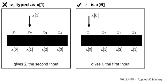
M01.1.4-F5
Wrong beside right. Python counts positions from 0, so the first item is x[0].
“\(x_1\) is x[1] in Python.”
x[1] is the item at position 1, counting from 0: the second input. \(x_1\) is x[0], and in general \(x_i\) is x[i - 1]. A slip like this often runs without any error message, because x[1] is a perfectly good item, just the wrong one. That is what makes it hard to spot.
“\(\hat{y}\) and \(y\) are the same thing.”
\(y_i\) is the true value and \(\hat{y}_i\) is the model’s guess. Their difference, \({\hat{y}_i - y_i}\), is the error that training tries to make small. Drop the hat and you have claimed the model is never wrong.
“\({\approx}\) is just a lazy \({=}\).”
\({\sqrt{2} \approx 1.4142}\) is true, but \({1.4142^2 = 1.99996164}\), not 2. Writing \({=}\) would claim something false. Use \({\approx}\) whenever a number has been rounded.
“A Greek letter always means the same thing.”
\(\pi\) is 3.14159… in geometry and a policy in reinforcement learning; \(\sigma\) is a standard deviation in statistics and the sigmoid function in ML01.6. Every good text defines its symbols: read those definitions first.
Check yourself
Recall
1. Read \({\hat{y}_i = w x_i + b}\) aloud, and name its parameters.
Show answer
“y-hat sub \(i\) equals \(w\) times x sub \(i\), plus \(b\)”. The parameters are \(w\) and \(b\).
2. A list has \({n = 4}\) items. What are its first and last items called in maths, and in Python?
Show answer
\(x_1\) and \(x_4\) in maths; x[0] and x[3] in Python.
3. What does a hat on a letter mean, and what does a bar mean?
Show answer
A hat marks a value made by a model, such as the prediction \(\hat{y}_i\). A bar marks a mean, such as \(\bar{x}\).
4. Which Greek letter does this site use for the learning rate, and which for all the parameters of a model?
Show answer
\(\eta\) (eta) for the learning rate and \(\theta\) (theta) for all the parameters.
5. Find the mean of 2, 4 and 9.
Show answer
Add them and divide by 3: \({(2 + 4 + 9)/3}\) is \(15/3\), which is 5.
Exercises
1.★ With \({w = 1.4}\) and \({b = 0.5}\), compute \({wx + b}\) for \({x = 0}\), \({x = 2.5}\) and \({x = 10}\), and read each line aloud.
Show solution
At \({x = 0}\): \({1.4 \times 0 + 0.5 = 0.5}\), read “1.4 times nought, plus 0.5, equals 0.5”. At the input 0 the prediction is the bias itself.
At \({x = 2.5}\): \({1.4 \times 2.5}\) is 3.5, and \({3.5 + 0.5 = 4}\). Read “1.4 times 2.5, plus 0.5, equals 4”.
At \({x = 10}\): \({1.4 \times 10}\) is 14, and \({14 + 0.5 = 14.5}\). Read “1.4 times 10, plus 0.5, equals 14.5”.
The middle one is worth noticing: at the mean input \({\bar{x} = 2.5}\) the model predicts 4, which is \(\bar{y}\).
2.★★ For the course’s data, write out the errors \({e_i = \hat{y}_i - y_i}\) for \({i = 1, 2, 3, 4}\). Find the mean of the errors and the mean of the predictions.
the same as \(\bar{y}\). That fits: the predictions are the targets plus the errors, and the errors add up to 0.
3.★★★ Show, with letters, that if \({\hat{y}_i = w x_i + b}\) for every \(i\), then the mean of the predictions is \({w\bar{x} + b}\). Check the result on the course’s numbers.
Show solution
First add up the predictions, putting in the formula for each one:
\[
\begin{aligned}
& \hat{y}_1 + \dots + \hat{y}_n \\
&\quad = (w x_1 + b) + \dots \\
&\qquad {} + (w x_n + b) \\
&\quad = w (x_1 + \dots + x_n) + n b \\
&\quad = n w \bar{x} + n b .
\end{aligned}
\]
The fourth line gathers the terms \(w x_i\) and takes out their common factor \(w\) (the distributive law), and gathers the \(n\) copies of \(b\) into \(nb\). The last line uses the definition of the mean, multiplied through by \(n\): \({x_1 + \dots + x_n = n\bar{x}}\). Now divide the total by \(n\) to get the mean of the predictions:
\[
\frac{n w \bar{x} + n b}{n} = w\bar{x} + b .
\]
Check: \({1.4 \times 2.5 + 0.5 = 4}\), and exercise 2 found the mean of the predictions to be 4.
Summary card
Every symbol in a formula has a job: data, parameter, constant or result.
M01.1.4-F1
Read it aloud, part by part.
\(x_1, \dots, x_n\) is a list; \(x_i\) is its \(i\)-th item. Python counts from 0: \(x_i\) is x[i - 1].
A hat is a prediction, \(\hat{y}_i\); a bar is a mean, \(\bar{x}\).
\(\bar{x}\) is the sum of the items divided by \(n\), and the differences \({x_i - \bar{x}}\) add up to 0.
For the course’s data, \({\hat{y} = 1.9, 3.3, 4.7, 6.1}\), \({\bar{x} = 2.5}\) and \({\bar{y} = 4}\).
Sources and next steps
Sources. Each was opened and checked against this lesson on 12 November 2026.
Jay Abramson and others, Algebra and Trigonometry 2e, OpenStax, Section 13.1, Sequences and Their Notations. It writes the terms of a sequence \(a_1, a_2, a_3, \dots, a_n\), calls \(a_1\) the first term, and uses the number subscript to give a term’s position.
Barbara Illowsky, Susan Dean and others, Introductory Statistics 2e, OpenStax, Section 12.3, The Regression Equation: \(\hat{y}\) is read “y hat” and is the estimated value of \(y\), and \(\bar{x}\) and \(\bar{y}\) are the sample means of the \(x\) and \(y\) values.
Ian Goodfellow, Yoshua Bengio and Aaron Courville, Deep Learning, Notation. Element \(i\) of a vector is written with a subscript, “with indexing starting at 1”; the page also uses \(\sigma\) for the logistic sigmoid, \(\mu\) for the mean of a Gaussian and \(\theta\) for the parameters of a function.
Python Software Foundation, An Informal Introduction to Python, The Python Tutorial, Sections 3.1.2 and 3.1.3 (Python 3.12): strings are indexed with the first character at index 0, and lists are indexed the same way. NumPy, numpy.mean: the arithmetic mean is the sum of the elements divided by the number of elements.
Next. The module ends here. Course module M01.2, Coordinates and a first look at vectors, crosses two number lines to make the plane and draws these four data points on it.